All About Search Algorithms

In progress

TO-DO:

• Refine RRT, RRT-Connect, RRT*
• POMDP
• Multi-robot planning

Graph Search Problem

Once a robot converts the environment into a discrete representation, whether by grid decomposition, Voronoi skeletons, adaptive cell decompositions, or lattices, the planning problem becomes a classical least-cost path search on a graph. Each state represents a robot configuration, and each edge carries a transition cost, typically the motion cost between configurations.

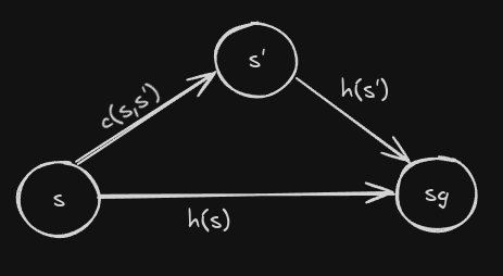
The goal of search is to compute a path from a designated start state $s_{start}$ to a goal state $s_{goal}$ that minimizes cumulative edge cost. Many search algorithms operate by estimating or computing the optimal cost-to-come, expressed as:

\[g(s) = \min_{s'' \in \text{pred}(s)} \left[ g(s'') + c(s'', s) \right]\]

Here, $g(s)$ is the minimum cost from start to $s$, $c(s’‘,s)$ is the cost of transitioning from predecessor $s’’$ to $s$, and the recursion states that the optimal cost-to-come is obtained by choosing the predecessor that yields the cheapest total.

Because this recurrence defines a dynamic programming relation, the overall optimal path can be reconstructed greedily by backtracking from the goal using the minimizing predecessor:

\[s' = \arg\min_{s'' \in \text{pred}(s)} \left[ g(s'') + c(s'', s) \right]\]

This backtracking forms the optimal path even though search expands states in the forward direction.

A*

A* expands states in increasing order of:

\[f(s) = g(s) + h(s)\]

where

• $g(s) =$ best-known cost from start to $s$
• $h(s) =$ admissible heuristic estimating $s$ to goal

A consistent heuristic ensures that every state g-value is optimal exactly at the moment the state is expanded. That is the heart of A’s correctness proof: A never has to revisit or “fix” a g-value later, because consistency ensures no cheaper path will ever emerge after expansion.

The algorithm expands only states whose f-values are competitive with the optimal path to the goal. This is why A* is so efficient: it prunes everything that cannot possibly lead to the optimal solution.

Pseudocode:

main()
g(s_start) = 0; all other g-values = INF;
OPEN = {s_start};
computePath();

computePath()
while(s_goal is not expanded and OPEN != 0)
	remove s with the smallest [f(s) = g(s)+h(s)] from OPEN;
	insert s into CLOSED;
	for every successor s’ of s such that s’ not in CLOSED:
		if g(s’) > g(s) + c(s,s’):
			g(s’) = g(s) + c(s,s’);
			insert s’ into OPEN;

For every expanded state $g(s)$ is optimal. For every other state, $g(s)$ is an upper-bound.

A* performs provably minimal number of state expansions required to guarantee optimality – optimal in terms of the computations.

Multi-Goal A*

Many robotic tasks require a path to any one of multiple possible goals. Examples include:

• picking the best parking spot out of many,
• intercepting a moving target at any predicted point along its trajectory,
• exploration where several frontier cells represent different potential “completion” points.

The key insight is that A* does not need special logic for multiple goals. Instead, introduce an imaginary super-goal connected to each real goal with zero-cost edges.

Once we add the super-goal node, the problem becomes identical to standard A*: now we just search from the start to this single super-goal. The f-values handle all the rest.

This equivalence is mathematically correct because:

\[c^*(s_{\text{start}}, g_{\text{imag}}) = \min_i c^*(s_{\text{start}}, g_i) \quad \text{(zero-cost jump at the end)}\]

This works even with unequal goal quality — e.g., one parking spot may be worse than another. In that case each real goal is connected to the imaginary super-goal with an edge equal to the additional cost (e.g., “goal cost”), so A* automatically prefers the better goal.

The transformed graph remains admissible for the original problem, and A* still returns the optimal plan among all candidate goals.

To incorporate this, assign each goal a terminal cost $w_i$, and connect to the imaginary goal with edge cost $w_i:$

\[c(g_i, g_{\text{imag}}) = w_i\] \[c^*(s_{\text{start}}, g_{\text{imag}}) = \min_i \left[ c^*(s_{\text{start}}, g_i) + w_i \right]\]

Weighted A*

Weighted A* modifies the f-value:

\[f(s) = g(s) + \epsilon h(s)\]

with $\epsilon>1$.

By inflating the heuristic weight, the search biases more strongly toward the goal, reducing exploration of irrelevant detours. This yields an $\epsilon-$suboptimal algorithm, meaning:

\[\text{cost(solution)} \le \epsilon \cdot \text{cost(optimal solution)}\]

Why it works?

The quality of A*’s heuristic is captured by the difference:

\[e(s) = h(s) - h^*(s)\]

• $h(s):$ the heuristic estimate
• $h^*(s):$ the true cost-to-go
• $e(s):$ indicates how much the heuristic underestimates the real cost

Since heuristics must be admissible, $e(s)$ is non-positive (never > 0).

Regions where the heuristic underestimates a lot (very negative $e(s)$) form local minima in the error landscape. A* expands many states inside these “deep valleys” because the f-values look artificially good.

A deep valley $\rightarrow$ many states look promising $\rightarrow$ A* wastes expansions.

Weighted A* modifies f-values:

\[f(s) = g(s) + \epsilon h(s), \quad \epsilon > 1\]

Multiplying the heuristic:

• raises the $h(s)$
• makes the heuristic less conservative
• makes error $e(s) = \epsilon h(s) - h^*(s)$
• turns deep valleys into shallow ones

This reduces the “funnel effect” and helps the search avoid unnecessary exploration.

Because local minima become shallow:

• A* commits sooner toward the goal
• explores fewer misleading states
• avoids wasting time in heuristic dips

Thus the search becomes directed, not exploratory.

No one currently knows precisely how the set of expanded states depends on the heuristic landscape. This remains an active research topic in heuristic search.

Backward A*

Backward A* simply reverses the direction of search. Instead of searching forward from the start, it starts from the goal and expands backwards:

Pseudocode:

main()
g(s_goal) = 0; all other g-values = INF;
OPEN = {s_goal};
computePath();

computePath()
while(s_start is not expanded and OPEN != 0)
	remove s with the smallest [f(s) = g(s)+h(s)] from OPEN;
	insert s into CLOSED;
	for every predecessor s’ of s such that s’ not in CLOSED:
		if g(s’) > c(s',s) + g(s):
			g(s’) = c(s',s) + g(s);
			insert s’ into OPEN;

Heuristics

The efficiency of A* is driven entirely by how good your heuristic is. A heuristic represents an “optimistic guess” of how far we still are from the goal. When the heuristic is informative, A* expands only a small portion of the graph; when the heuristic is uninformative, A* degenerates toward Dijkstra, expanding almost everything.

The formal requirement for heuristics in A* is admissibility: the heuristic must never overestimate the true cost-to-go. In symbolic terms:

\[0 \le h(s) \le c^*(s,s_{goal})\]

where $c^*(s,s_{goal})$ is the minimal cost from $s$ to $s_{goal}$.

This ensures that A* never prunes or skips any potentially optimal path. But admissibility alone does not guarantee efficiency. For A* to run fast, the heuristic must not only be admissible, but also consistent (monotone). Consistency means:

\[h(s_{goal}, s_{goal})=0\] \[h(s) \le c(s,s') + h(s')\]

for every $s\ne s_{goal}$ and its successors $s’.$

Admissibility provably follows from consistency and often (not always) consistency follows from admissibility.

Functions

For grid-based navigation:

• Euclidean distance
  • Admissable for 4-connected and 8-connected grid
• Manhattan distance: $h(x,y) = abs(x-x_{goal}) + abs(y-y_{goal})$
  • Admissable for 4-connected grid (perfect heuristic)
  • Inadmissable for 8-connected grid (Octile function is the perfect heuristic)
• Diagonal distance: $h(x,y) = max( abs(x-x_{goal}), abs(y-y_{goal}))$

Octile Heuristic:

In more complex spaces like a 3D lattice $(x,y,\theta)$ or high-DoF manipulators, a naïve heuristic becomes almost useless because it collapses the structure of the real problem into something too simple to guide search well.

A common and powerful strategy is to compute a lower-dimensional search to define a heuristic for a higher-dimensional state. For example, running a 2D Dijkstra search on the grid (starting from the goal) produces distances that account for real obstacles; these distances can then be used as heuristic values for every $(x,y,\theta)$ configuration. This improves guidance but can still fail in problems where orientation or arm constraints dominate the difficulty.

In many robotic tasks, even a sophisticated lower-dimensional heuristic is not enough because the true difficulty comes from complex geometric or kinematic constraints. In these cases, we often turn to inadmissible heuristics that violate the admissibility rule but encode meaningful structure—such as end-effector distance through obstacles or orientation differences of manipulated objects. These heuristics are informative but unsafe to use alone because they can lead A* into local minima or cause it to miss valid solutions.

Key Properties of Combining Heuristics

If two heuristics $h_1(s)$ and $h_2(s)$ are consistent, then using their maximum,

\[h(s) = \max(h_1(s), h_2(s))\]

remains consistent and therefore admissible. This is useful but extremely limited: the max operation destroys information, produces new local minima, and requires every heuristic to be admissible, which is unrealistic in high-dimensional robotics.

More generally, if heuristics are combined additively,

\[h(s) = h_1(s) + h_2(s)\]

the result is typically $\epsilon-$consistent, meaning the heuristic may overestimate by at most a bounded factor. Weighted A* is equivalent to using such $\epsilon-$consistent heuristics and guarantees

\[\text{cost(solution)} \le \epsilon \cdot \text{cost(optimal)}\]

Need for Multiple Heuristics

Real-world manipulation or navigation tasks often have many distinct modes of difficulty, where each heuristic is strong in some region but weak (or utterly misleading) in others. For instance:

• One heuristic might capture distance in the workspace.
• Another might encode object orientation costs.
• A third might describe arm retraction or clearance constraints.

No single heuristic, admissible or inadmissible, gives uniformly good guidance across the entire state space.

This motivates algorithms that can leverage many heuristics simultaneously without losing theoretical guarantees.

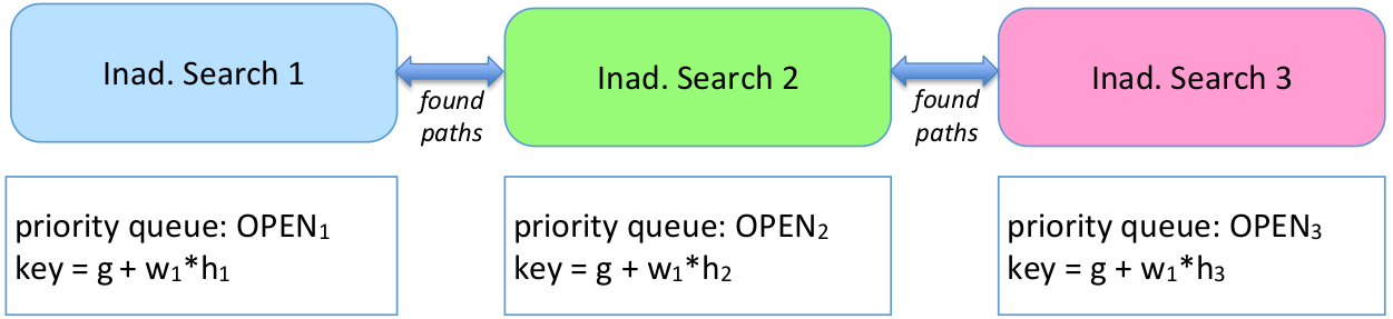
Multi-Heuristic A*

Version 1

• Given $N$ inadmissible heuristics
• Run $N$ independent searches
• Hope one of them reaches goal

Problems:

• Each search has its own local minima
• $N$ times more work
• No completeness guarantees or bounds on solution quality

Within the while loop of the ComputePath function:
	for i=1…N:
		remove s with the smallest [f(s) = g(s)+w1*h(s)] from OPENi ;
		expand s;

Version 2

• Given $N$ inadmissible heuristics
• Run $N$ independent searches
• Hope one of them reaches goal
• Share information (g-values) between searches

Within the while loop of the ComputePath function (CLOSED is shared):
	for i=1…N:
		remove s with the smallest [f(s) = g(s)+w1*h(s)] from OPENi ;
		expand s and also insert/update its successors into all other OPEN lists;

Benefits:

• Searches help each other to circumvent local minima
• States are expanded at most once across ALL searches

Remaining Problem: No completeness guarantees or bounds on solution quality

Version 3

• Given $N$ inadmissible heuristics
• Run $N$ independent searches
• Hope one of them reaches goal
• Share information (g-values) between searches
• Search with admissible heuristics controls expansions

Within the while loop of the ComputePath function 
(CLOSED is shared among searches 1…N. Search 0 has its own CLOSED):
	for i=1…N:
		if(min. f-value in OPENi ≤ w2* min. f-value in OPEN0 )
			remove s with the smallest [f(s) = g(s)+w1*hi(s)] from OPENi ;
			expand s and also insert/update its successors into all other OPEN lists;
		else
			remove s with the smallest [f(s) = g(s)+w1*h0(s)] from OPEN0 ;
			expand s and also insert/update its successors into all other OPEN lists;

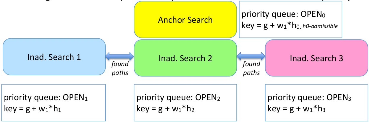
The algorithm runs $N+1$ parallel A*-like searches:

• Search 0: the anchor search using admissible $h_0$
• Search 1…N: searches using inadmissible heuristics $h_1, h_2,…,h_N$

Each search has its own OPEN list (priority queue).

But:

• searches 1…N share the same CLOSED list
• search 0 has its own CLOSED list
• all searches share g-values

If the inadmissible search is “good enough”: Search i’s best node looks promising enough compared to the anchor search.

\[\text{min}f_i \le w_2.\text{min}f_0\]

If the inadmissible search is not good enough: Search i’s best node is not competitive. Do not trust its heuristic right now.

\[\text{min}f_i > w_2.\text{min}f_0\]

Need for two weights:

• $w_1$ inflates heuristics inside each individual search (making $f=g+w_1h$)
• $w_2$ compares searches against the anchor and decides if inadmissible searches are allowed to expand

Together, they ensure:

\[\text{cost(solution)} \le w_1 w_2 \cdot \text{optimal cost}\]

• Searches 1…N (inadmissible): share a single CLOSED list
  • so no state is expanded more than once among all inadmissible searches
• Anchor search has a separate CLOSED list
  • so anchor may expand a state once, even if inadmissible searches already expanded it

So each state is expanded at most twice.

Interleaving Planning and Execution

In real-world robotics, planning is not a one-time activity. The robot must continuously update its plan while moving, because the world is not fully known beforehand, and conditions may change during execution.

Typical reasons why planning must be repeated are:

• The environment is only partially known (unknown obstacles revealed during motion).
• The environment might be dynamic (people, vehicles, or other robots moving).
• The robot may not follow its plan perfectly due to actuation or drift errors.
• Its state estimation may be imprecise, causing localization errors.

In such cases, the robot must be able to re-plan quickly instead of starting A* from scratch.

When a robot must plan repeatedly, there are three main approaches:

1. Anytime heuristic search — returns the best available solution within a time limit and keeps improving it.
2. Incremental heuristic search — speeds up repeated searches by reusing past search efforts, like g-values, OPEN lists, or search trees.
3. Real-time heuristic search — only plans a few steps ahead, executes them, then re-plans later.

Anytime Heuristic Search

A basic idea of Anytime search is to start with a fast, suboptimal solution and improve it as more time becomes available.

Weighted A* uses:

\[f(s) = g(s) + \epsilon \cdot h(s), \quad \epsilon > 1\]

• With large $\epsilon$, the solution is found quickly but may not be optimal.
• As $\epsilon$ approaches 1, the solution becomes optimal but search becomes slower.

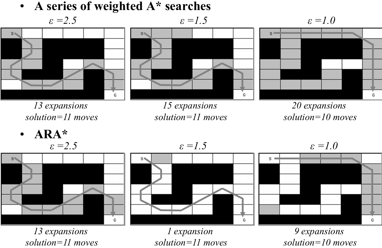
A simple but inefficient approach: run Weighted A* multiple times with decreasing $\epsilon$ ( $2.5 \rightarrow 1.5 \rightarrow 1.0$ ), restarting every time. But this is wasteful, because many values do not change between searches.

ARA: Anytime Repairing A

ARA* improves on this by reusing the results of previous searches, instead of restarting from scratch.

ARA* solves this by:

• Quickly returning a first solution using a high weight
• Reducing the weight step-by-step to improve solution quality
• Reusing previous g-values, OPEN lists, and search tree structure
• Avoiding needless re-expansions

Pseudocode:

main()
g(s_start) = 0; all other g-values = INF;
OPEN = {s_start};
computePathWithReuse();

all v-values are initially INF;
initialize OPEN with all overconsistent states;
computePathWithReuse()
while(f(s_goal) > minimum f-value in OPEN)
	remove s with the smallest [f(s) = g(s)+h(s)] from OPEN;
	insert s into CLOSED;
	v(s) = g(s);
	for every successor s’ of s such that s’ not in CLOSED:
		if g(s’) > g(s) + c(s,s’):
			g(s’) = g(s) + c(s,s’);
			insert s’ into OPEN;

\[g(s') = \text{min}_{s'' \in pred(s')}v(s'')+c(s'',s')\]

$OPEN:$ set of all states with $v(s) > g(s)$. All other states have $v(s)=g(s).$

ARA* keeps two cost values for each state:

• The current best-known cost $g(s)$
• The cost when the state was last expanded $v(s)$. If the state was never expanded, then its value is $INF$.

The difference between these two tells ARA* whether a state needs to be re-expanded under the new (lower) weight.

• Consistent: $v(s) = g(s)$

  The state’s value matches the last expansion. So no rework is needed.

• Overconsistent: $v(s) > g(s)$

  The state’s cost has improved since it was expanded. So it might need re-expansion.

• Underconsistent: $v(s) < g(s)$

  State’s cost has worsened (rare unless environment changes). So also needs to be fixed.

ARA* re-expands only the inconsistent states rather than the whole search space.

How ARA* Improves the Solution Without Restarting?

When the weight $\epsilon$ decreases:

1. ARA* inserts all inconsistent states into OPEN
2. It runs a Weighted-A*-like search again, but:
   • g-values remain
   • the old search tree remains
   • states that were consistent stay untouched
3. Expansion continues until:
   • A new solution with the smaller $\epsilon$ is found
   • No g-value can be further improved

This allows ARA* to give multiple solutions, each guaranteed to be within $\epsilon.$optimal.

At every iteration, ARA* guarantees:

\[\text{cost(solution)} \le \epsilon \cdot \text{cost(optimal)}\]

Pros:

ARA* saves time due to:

• Reusing previous g(s) values
• Reusing the previous OPEN list
• Only expanding inconsistent states
• Avoiding recomputation of the whole search tree
• Avoiding redundant expansions

Pseudocode using weighted A*:

main()
g(s_start) = 0; all other g-values = INF;
OPEN = {s_start};
while e ≥ 1
	CLOSED = {}; INCONS = {};
	computePathwithReuse();
	publish current e suboptimal solution;
	decrease e;
	initialize OPEN = OPEN U INCONS;

all v-values are initially INF;
initialize OPEN with all overconsistent states;
computePathWithReuse()
while(f(s_goal) > minimum f-value in OPEN)
	remove s with the smallest [f(s) = g(s)+eh(s)] from OPEN;
	insert s into CLOSED;
	v(s) = g(s);
	for every successor s’ of s:
		if g(s’) > g(s) + c(s,s’):
			g(s’) = g(s) + c(s,s’);
			if s' not in CLOSED then insert s’ into OPEN;
			otherwise insert s' into INCONS

if s' not in CLOSED then insert s’ into OPEN exists because in weighted A*, the g-values are not guaranteed to be optimal. So even if a successor has been expanded before, there is a chance that its g-value can be made better. Hence it is updated but it is not put in the OPEN list again because it has been expanded before.

In regular A*, the g-values are already optimal if the state is CLOSED, so they don’t need to be updated.

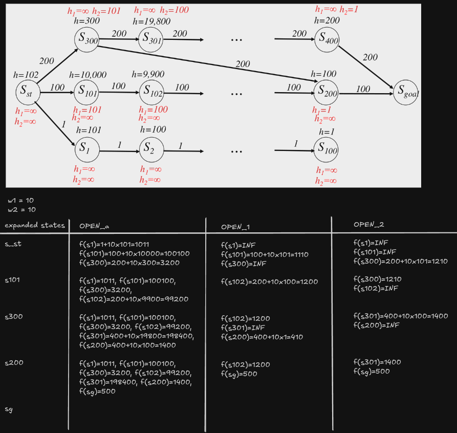
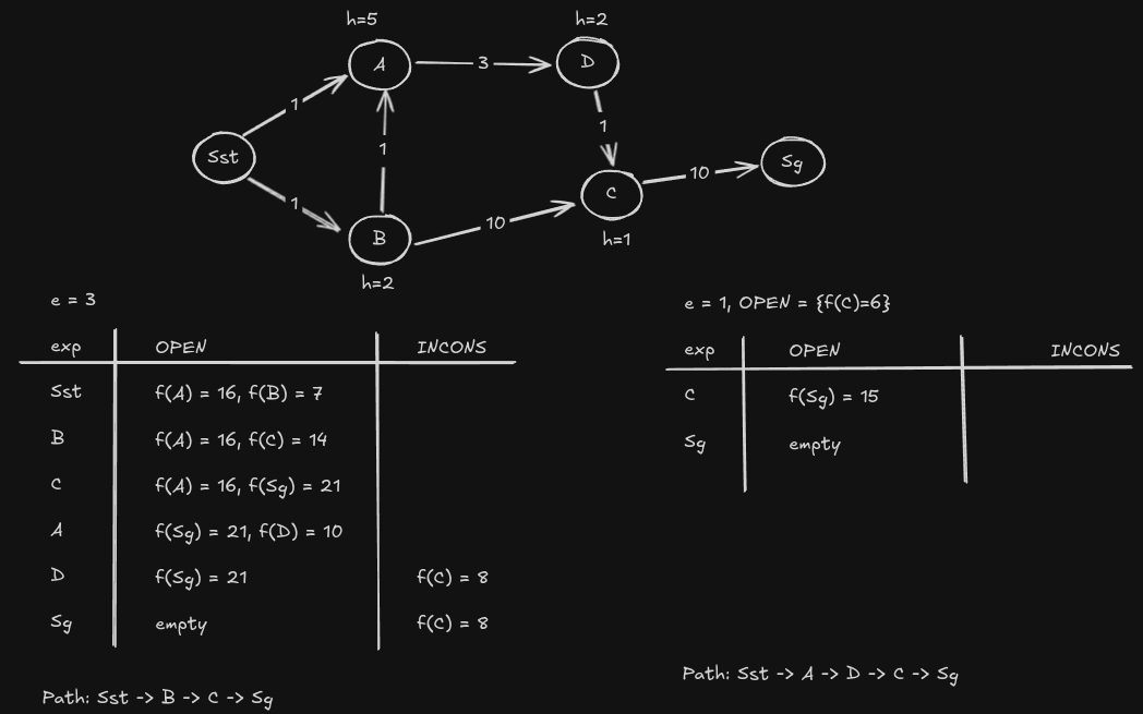
Example:

Real-Time Heuristic Search

Traditional A* and its variants assume that planning is completed before execution begins. This assumption breaks down in realistic robotics settings:

• The environment is often partially known, and important obstacles become visible only during execution.
• The world may be dynamic, forcing the robot to react immediately to avoid collisions.
• Robots experience imprecise motion and noisy localization, which invalidates long pre-computed plans.
• Some tasks require millisecond-level reactivity, making full-path planning infeasible.

Real-time search treats planning and acting as a continuous loop: gather sensor data → plan a few steps → execute one step → repeat.

Real-time search limits the amount of planning:

• At each iteration, the agent may expand only N nodes (where N is small and fixed).
• After that limited search, the agent chooses the next action that looks best.
• The agent then moves exactly one step, updates the map, and begins the next lookahead.

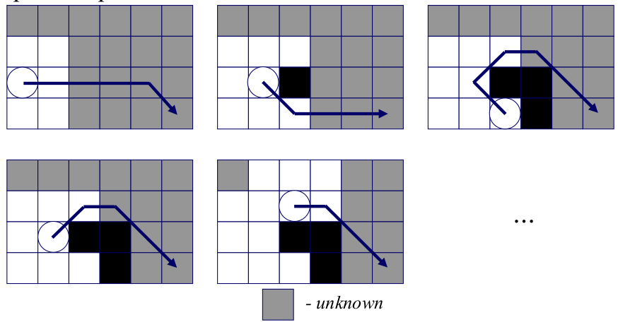
This approach ensures that the robot always responds in bounded time, even in unknown or rapidly changing environments. It never aims to produce a global path immediately; instead, it incrementally constructs a path through repeated short-range planning.

When the map is unknown, real-time search relies on the Freespace Assumption: All unexplored cells are assumed to be free until the robot’s sensors reveal otherwise. This lets the planner behave optimistically and aggressively move toward the goal. When the robot detects new obstacles, they are incorporated into the map and the next real-time search cycle adapts accordingly. The Freespace Assumption enables motion in unknown worlds but also creates the need for heuristic correction because the robot can fall into local minima where the heuristic dramatically underestimates real cost-to-go.

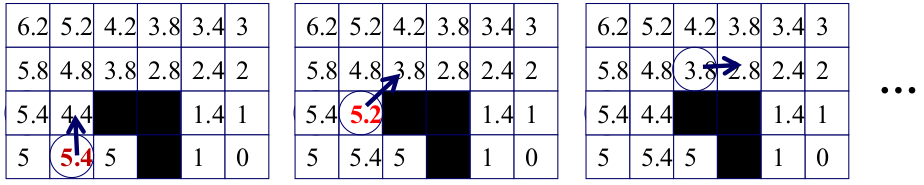
LRTA*: Learning Real-Time A*

At each iteration:

1. The agent evaluates all immediate successors $s’$ of the current state $s$ and moves to the minimum, as follows:

   \[s = \text{argmin}_{s' \in succ(s)}c(s,s')+h(s')\]

2. Before leaving state $s$, LRTA* updates the heuristic:

   \[h(s) \leftarrow \min_{s' \in succ(s)} \left( c(s, s') + h(s') \right)\]

This update increases the heuristic at states where the robot got stuck, reducing the attractiveness of that region. Over many steps, LRTA* guarantees that the heuristic monotonically increases toward the true cost-to-go.

LRTA* thus learns a better heuristic online and ensures eventual escape from every local minimum.

Convergence Properties of LRTA*

LRTA* guarantees that the robot will reach the goal in a finite number of steps:

• If the graph is finite, action costs are positive, and a solution exists, LRTA* will reach the goal in finite time.
• It will never oscillate infinitely because heuristic updates eliminate the cause of repeated cycles.
• The learned heuristic converges to a consistent, admissible function that reflects encountered terrain.
• All actions are reversible.
• h-values remain admissible and consistent.

This makes LRTA* suitable for unknown environments where the robot must “feel its way” toward the goal.

Multi-Step Lookahead in LRTA*

Basic LRTA* examines only immediate neighbors, which can be shortsighted.

A more powerful variant performs an N-step lookahead:

• Expand up to N nodes using a limited search (A*, BFS, or Dijkstra-like expansion).
• Compute locally optimal g-values for these nodes.

• Use local dynamic programming updates:

  \[h(s) = \min_{s' \in succ(s)} \left( c(s, s') + h(s') \right)\]

• Move on path to the state $s$

  \[s = \text{argmin}_{s' \in OPEN}g(s')+h(s')\]

This deeper lookahead reduces the number of heuristic updates needed and helps the robot anticipate dead ends earlier.

RTAA*: Real-Time Adaptive A*

RTAA* is a more efficient form of heuristic learning suitable for large-scale real-time robotics. Instead of performing full DP updates like LRTA, RTAA computes a single batch update per cycle. After expanding a bounded search frontier during lookahead, RTAA* identifies the most promising frontier node $s^*$ (the one minimizing $g+h$), and updates the heuristics of all expanded states using:

\[h(u) \leftarrow f(s^*) - g(u)\]

PRM

For manipulation tasks, the robot’s configuration is a vector of joint angles $Q={q_1,\ldots,q_n}$, which defines a point in a continuous, high-dimensional space called configuration space (C-space). Planning requires computing a continuous path from $Q_{start}$ to $Q_{goal}$ that satisfies all constraints:

• Joint limits
• No collisions with obstacles
• No self-collisions

A direct grid discretization of this space becomes infeasible because the number of grid cells grows exponentially with dimension. Although resolution-complete planners guarantee completeness and quality bounds, they become computationally intractable in 6- to 12-dimensional spaces typically encountered in manipulation.

Sampling-based methods exploit the insight that although the configuration space is high-dimensional, the free space is continuous and “benign”, meaning a sparse set of samples can capture enough structure of the environment to allow feasible paths to be found.

Overview

PRMs operate in two phases:

Preprocessing Phase (Learning Phase)

A roadmap graph $G$ is built using random samples in $C_{free}$. Each sample is connected to nearby samples through short, locally planned paths, typically straight-line interpolation in joint space.

Query Phase

Given arbitrary start and goal configurations:

1. Connect both to the roadmap using a local planner.
2. Run a graph search (A, Dijkstra, Weighted A) on the augmented roadmap.

If the roadmap is sufficiently dense, start and goal will connect to the same component of the graph, making a valid continuous path available.

A single roadmap can answer many queries efficiently, which is why PRMs are well suited for multi-query environments such as manipulation in structured spaces.

Preprocessing Phase

Sampling: We repeatedly generate random configurations $\alpha(i)$ in $C_{free}$. Each sample must satisfy all constraints (no collisions, valid joint limits). Samples can be uniform or follow more sophisticated biasing strategies.

Adding Vertices: Whenever a sample lies in free space, it is added as a vertex in the roadmap graph.

Neighborhood Selection: For each new sample, we identify a set of nearby vertices in the existing graph. Some commonly used neighborhood definitions:

1. K nearest neighbors (distance in configuration space)
2. Nearest neighbor in each connected component of the roadmap
3. All vertices within a radius $r$

The goal is to avoid creating too many edges while guaranteeing connectivity.

Connecting Neighbors: For each neighbor vertex $q$, we call a local planner to determine whether a smooth, collision-free path exists between $\alpha(i)$ and $q$. Even a simple straight-line interpolation in joint space is often sufficient. If this local plan is collision-free, an edge is added to the graph.

Connected Components: The roadmap grows organically, gradually connecting isolated components until the free space is covered well enough to support queries.

Pseudocode:

BUILD_ROADMAP
   G.init();  i ← 0;
   while i < N
       if α(i) ∈ C_free then
           G.add_vertex(α(i));  i ← i + 1;
           for each q ∈ NEIGHBORHOOD(α(i), G)
               if ( (not G.same_component(α(i), q)) and CONNECT(α(i), q) ) then
                   G.add_edge(α(i), q);

Query Phase: Using the Roadmap

Once the roadmap is built, answering queries becomes fast:

1. Given $q_I$ and $q_G$, connect each to nearby vertices in the roadmap using the same local planner
2. Insert both into the graph as temporary nodes
3. Use a shortest-path algorithm such as Dijkstra’s or A*
4. If both nodes lie in the same connected component, the resulting path is a valid collision-free motion

Sampling Strategies

Uniform sampling is the simplest approach but can be highly inefficient. Certain regions of configuration space — such as narrow passages between obstacles — have extremely small measure and are rarely sampled. PRMs address this with multiple sampling strategies:

1. Uniform sampling: Samples drawn uniformly from free space. Fast and easy, but may fail to represent narrow corridors adequately.
2. Connectivity-Based Sampling: Sample existing vertices with probability inversely proportional to how well-connected they are. Poorly connected vertices (likely in narrow regions) get sampled more often, increasing coverage of difficult areas.
3. Obstacle-Biased Sampling: Sampling is biased toward the boundary of obstacles. This helps generate samples near constraints where the roadmap usually needs more detail.
4. Gaussian Sampling: Gaussian sampling generates small clusters of samples around a chosen point. If one sample lies in collision and another lies in free space, the free one is kept. This produces samples near obstacle boundaries without explicitly detecting the boundary.
5. Bridge Sampling: Sampling $q_1, q_2, q_3$ from a Gaussian and keeping the middle configuration if it is in free space but neighbors are in collision. This helps find narrow passages effectively.
6. Sampling Away from Obstacles: Useful in cluttered environments where the robot needs large free areas well represented.

Each sampling heuristic targets a failure mode of uniform sampling, making the resulting roadmap more robust.

Pros and Cons

PRMs excel in multi-query, high-dimensional spaces:

Strengths

• Extremely efficient once the roadmap is built
• Scales well to high-dimensional C-spaces
• Easy to integrate with collision checkers and kinematic constraint solvers
• Probabilistically complete

Weaknesses

• Roadmap building can be expensive initially
• Difficult to handle dynamic environments (PRM is primarily offline)
• Narrow passages require careful sampling strategies
• Connectivity depends heavily on sample quality

RRT

RRTs are particularly effective for single-query planning problems where a robot must find a feasible path between a specific start and goal configuration but does not expect to reuse planning work later. They scale well to high-dimensional configuration spaces and do not require a preprocessing phase. Compared to PRMs, RRTs sacrifice optimality but gain significant speed and robustness, especially when collision checking is expensive or the environment is cluttered.

Basic Structure

An RRT begins with a tree whose root is the start configuration. At each iteration, the planner draws a random configuration from the configuration space and finds the closest node in the tree. Instead of jumping directly to the sample, the algorithm takes only a small step toward it. This step is usually a straight-line interpolation in configuration space. If this short motion is collision-free, the new configuration is added to the tree.

This fundamental operation is the EXTEND operator. Conceptually, EXTEND tries to walk from a known configuration toward a random sample by a limited distance. This simple mechanism produces a tree that organically spreads into every region of the free space, with more growth where space is wide open and less growth in constrained areas.

The algorithm terminates when the tree grows sufficiently close to the goal, or when a direct local connection to the goal becomes feasible.

Psuedocode:

BUILD_RRT
  T.init(q_init);
  for k = 1 to K
      q_rand ← RANDOM_STATE();
      EXTEND(T, q_rand);
      
EXTEND(T, q):
      q_near ← NEAREST_NEIGHBOR(q, T);
      q_new  ← EXTEND(q_near, q);
      if q_new ≠ NULL then
          T.add_vertex(q_new);
          T.add_edge(q_near, q_new);
          if q_new = q_goal then
              return PATH(T, q_goal);
  return PATH_NOT_FOUND;

Limitations

Although RRTs are powerful explorers, they do not compute optimal or even high-quality paths. Because the algorithm grows outward from the start without explicitly optimizing anything, the resulting path is usually long, jagged, and geometrically irregular. Once a branch is created, the tree structure restricts future updates; the planner cannot easily reorganize previous decisions.

As a result, RRTs tend to lock themselves into a single homotopy class early on. They cannot “undo” their earlier tree structure, so even with more computation, the path does not improve. This makes standard RRT a great planner for fast feasibility but a poor choice for optimal path quality.

RRT-Connect: A Faster Bi-Directional Variant

RRT-Connect significantly accelerates planning by growing two trees simultaneously: one from the start configuration and one from the goal. At each iteration, a random sample is drawn, and one tree grows toward it using the standard EXTEND step. Once that extension succeeds, the algorithm immediately attempts to “pull” the other tree toward the newly created node.

This “aggressive connection” uses a CONNECT operation, which repeatedly performs EXTEND toward the same sample until either a collision is detected or the sample is reached. The result is a strong contraction motion: the two trees attempt to meet in the middle as fast as possible.

RRT-Connect tends to find feasible paths much faster than basic RRT. It inherits the same exploration bias and probabilistic completeness, but because of bi-directional growth and aggressive connection, it usually solves hard planning problems in far fewer expansions. However, like RRT, it does not produce optimal solutions.

The mechanics of EXTEND can be written as:

\[q_{\text{new}} = q_{\text{near}} + \varepsilon \cdot \frac{q_{\text{rand}} - q_{\text{near}}}{|q_{\text{rand}} - q_{\text{near}}|}\]

The algorithm adds $q_{new}$ to the tree only if the local connection segment:

\[\tau(s) = q_{\text{near}} + s(q_{\text{new}} - q_{\text{near}}), \quad s \in [0,1]\]

lies entirely inside $C_{free}.$

This geometric structure ensures the tree grows smoothly rather than in erratic jumps.

Pseudocode:

RRT_CONNECT(q_start, q_goal, N, ε):
    T_start.init(q_start)
    T_goal.init(q_goal)

    for k = 1 to N:
        q_rand ← SAMPLE_CONFIG()

        # 1) Grow T_start toward the random sample
        if EXTEND(T_start, q_rand, ε) ≠ TRAPPED:
            q_new ← LAST_ADDED_VERTEX(T_start)

            # 2) Try to CONNECT T_goal toward q_new aggressively
            if CONNECT(T_goal, q_new, ε) = REACHED:
                return EXTRACT_PATH_BIDIRECTIONAL(T_start, T_goal, q_new)

        SWAP(T_start, T_goal)    # alternate which tree is "start" vs "goal"

    return FAILURE

EXTEND(T, q_target, ε):
    q_near ← NEAREST_NEIGHBOR(T, q_target)
    q_new  ← STEER(q_near, q_target, ε)

    if COLLISION_FREE(q_near, q_new):
        T.ADD_VERTEX(q_new)
        T.ADD_EDGE(q_near, q_new)
        if q_new = q_target:
            return REACHED
        else:
            return ADVANCED
    else:
        return TRAPPED

CONNECT(T, q_target, ε):
    status ← ADVANCED
    while status = ADVANCED:
        status ← EXTEND(T, q_target, ε)
    return status

Why RRT Paths Need Smoothing

Because RRTs grow by random exploration, the final paths are rarely smooth. They often zig-zag through space inefficiently. A common remedy is the short-cutting technique, which repeatedly attempts to bypass intermediate vertices on the path by checking whether the straight-line segment between two non-adjacent configurations is collision-free.

If the shortcut succeeds, the interior of the path is replaced with the direct link:

\[\text{if } \texttt{CONNECT}(q_i, q_j) = \text{free} \quad\Rightarrow\quad \text{replace segment }( q_i \to q_{i+1} \to \dots \to q_j ) \text{ with } (q_i \to q_j)\]

This tends to produce significantly shorter and smoother paths while keeping computation lightweight.

RRT*

RRT* was introduced to address the largest limitation of standard RRT: its inability to improve path quality over time. RRT* modifies the tree structure so that every new sample can potentially improve not just its own branch but also the structure of the nearby tree.

When a new node $x_{new}$ is added:

1. Parent Selection: RRT* considers all tree nodes within a radius $r(n)$ around $x_{new}$. Among these candidates, it chooses as parent the neighbor that minimizes the total path cost:

   \[x_{\text{parent}} = \arg\min_{x \in X_{\text{near}}} \big( \text{Cost}(x) + c(x, x_{\text{new}}) \big)\]

2. Rewiring:

   After adding $x_{new}$, the planner checks whether using $x_{new}$ as a parent would reduce the cost of any neighboring nodes. If so, those nodes are “rewired” to point to $x_{new}$, improving the overall tree.

The rewiring step is the critical innovation: it continuously reorganizes the tree as new samples arrive, allowing the planner to refine earlier decisions instead of being trapped by them.

Asymptotic Optimality of RRT*

RRT* is asymptotically optimal, unlike RRT or RRT-Connect.

As the number of samples $n$ approaches infinity:

\[\lim_{n \to \infty} \text{Cost}( \text{best path from RRT}^* ) = \text{Cost}( \text{optimal path} )\]

This result is provable and depends on choosing the neighbor radius:

\[r(n) = \gamma \left( \frac{\log n}{n} \right)^{1/d}\]

where $d$ is the dimension of the configuration space.

Under this radius schedule, the tree becomes dense enough to guarantee optimal connections while still maintaining computational efficiency.

Trade-Offs Between RRT, RRT-Connect, and RRT*

There is a clear computational-optimality trade-off between these methods:

• RRT is extremely fast and good at finding any feasible path, but provides very low path quality.
• RRT-Connect is usually the fastest at finding a feasible path, especially in cluttered spaces.
• RRT* is slower per iteration but continuously improves the solution, eventually reaching the optimum.

In practice, the choice depends on the task:

• For real-time feasibility (e.g., robot moving through unknown space), RRT or RRT-Connect is preferred.
• For motion tasks requiring precise, smooth, or cost-minimal paths (e.g., manipulation, surgical robots), RRT* provides the needed optimality.

Markov Property

In search-based planning, the Markov property means: When you stand in a state $s$, everything you need to decide – what successors you can go to and what they will cost – is fully determined by the current state only, not by how you got there.

So:

\[\text{succ}(s) = \text{function of } s\] \[c(s, s') = \text{function of } (s, s'), \quad s' \in \text{succ}(s)\]

No “memory” of the previous path is allowed in $succ$ or $c$ (i.e., no dependence on the history of the path leading up to it).

Algorithms like Dijkstra, A*, dynamic programming, etc., assume that if you reach the same state again with higher cost, that path is always worse for the future. This is only true if the future behavior (successors and costs) depends only on the state, not on the path you took.

If the Markov property is broken:

• You might incorrectly prune states
• The algorithm can become incomplete (miss a solution) or sub-optimal

Independent vs Dependent Variables

Each search state $s$ contains a set of variables:

\[X(s) = \{ X_{\text{ind}}(s), X_{\text{dep}}(s) \}\]

Independent variables $X_{ind}(s)$:

• These define the state identity
• Two states are the same if and only if their independent variables are equal

\[s = s' \quad \text{iff} \quad X_{\text{ind}}(s) = X_{\text{ind}}(s')\]

Dependent variables $X_{dep}(s)$:

• Variables derived from the independent variables
• Used for successor generation, cost computation, heuristics, collision checks

The Markov property holds if dependent variables depend only on the independent ones:

\[X_{\text{dep}}(s) = f\big(X_{\text{ind}}(s)\big)\]

This means the planner can fully determine successors, transition costs, valid or invalid states, just from the current state itself.

Markov property is violated when you compute dependent variables using history:

\[X_{\text{dep}}(s) = f\big(X_{\text{ind}}(s), \text{history}\big)\]

Incompleteness

Incompleteness arises when your state representation or successor function violates the assumptions needed for graph search. It can happen for three major reasons:

• Incorrect state definition (missing independent variables)
• Dependent variables rely on history
• Successor generation fails to enumerate all possible transitions

To guarantee completeness:

• Include every future-relevant variable in $X_{ind}$
• Ensure dependent variables are pure functions of $X_{ind}$
• Ensure successor generation is fully determined
• Ensure edge costs depend only on $(s,s’)$

Dominance

Dominance is a pruning rule used in optimal search to reduce the number of states explored. The basic idea is that if two states represent the exact same situation, but one reached that situation with a lower g-value, and both share the same future possibilities, then the more expensive state can be discarded. This makes the search faster without losing optimality.

Two states can only be compared if they are identical in all independent variables:

\[X_{\text{ind}}(s_1) = X_{\text{ind}}(s_2)\]

If they differ in any independent variable, then they cannot dominate each other.

Dominance only works if independent variables fully determine all future successors and costs. That is the Markov property.

\[\text{succ}(s) = f(X_{\text{ind}}(s)), \quad c(s,s') = g(X_{\text{ind}}(s), X_{\text{ind}}(s'))\]

Task Planning

Task planning is a branch of robotics that deals with reasoning about high-level actions — actions that manipulate objects, change symbolic states of the world, and achieve complex goals. Unlike motion planning, which concerns itself with geometric paths and kinematic feasibility, task planning is fundamentally symbolic. It focuses on how the world can be transformed step-by-step through discrete, logically defined actions.

Task planning involves deciding what sequence of actions a robot must perform to accomplish a goal. These actions may involve picking objects up, stacking them, assembling parts, or performing multi-step procedures such as constructing a birdcage. The key challenge is not continuous robot motion but rather logical ordering: which actions must precede others, what dependencies exist, and how actions change the state of the world.

Blocksworld Example

One of the most famous examples in symbolic AI is Blocksworld. In this environment, various blocks can be stacked on one another or placed on a table. The robot’s task is to transform an initial arrangement of blocks into some desired configuration.

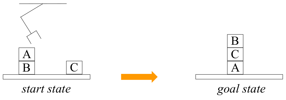
For instance, consider a start state where block A sits on block B, and block C sits on the table. The goal state may require placing C on A, and A on the table. The core challenge is deciding in what order the robot must move blocks to reach this arrangement. Movement is constrained — for example, the robot can only move blocks that have no other block on top of them.

The key insight is that Blocksworld is purely symbolic. The robot does not care about precise coordinates or continuous motion but instead about discrete relationships like:

• “On(A, B)”
• “Clear(A)” (nothing is stacked on top of A)
• “Block(C)” (C is a movable block)

These predicates define the symbolic state of the world.

Representing Blocksworld as a State-Space Graph

To use search algorithms, we must represent Blocksworld as a graph where each node is a symbolic state and edges correspond to actions. A state is simply the collection of all true statements (predicates) about the world at that moment. For example:

\[\text{State} = { \text{On(A, B)}, \text{On(B, Table)},\ \text{On(C, Table)},\ \text{Clear(A)},\ \text{Clear(C)},\ \text{Block(A)},\ \text{Block(B)},\ \text{Block(C)} }\]

Actions such as Move(b, x, y) transform one state into another by modifying these predicates. Each action has preconditions that must be true before it can be executed (e.g., the block must be clear, and the target must be clear) and effects that describe how the state changes. If action preconditions are satisfied, the action is applicable, and it creates a successor state in the search graph.

This transforms Blocksworld into a state-space search problem, where A* or breadth-first search can discover the shortest action sequence from the start state to any state matching the goal description.

STRIPS

STRIPS (Stanford Research Institute Problem Solver) provides a structured way to define symbolic planning problems. It describes a planning problem using three components: state representation, goal representation, and action representation.

State Representation in STRIPS

A state is represented as a conjunction of positive literals, meaning it is a set of statements about the world that are true. For example:

\[\text{On(A,B)} \wedge \text{On(B,Table)} \wedge \text{Clear(A)} \wedge \text{Block(A)} \wedge \text{Block(B)}\]

Crucially, STRIPS uses the closed-world assumption: any fact not listed in the state is assumed to be false. This means we only list what is true; everything else is false by default.

Goal Representation in STRIPS

Goals in STRIPS are also defined as a conjunction of positive literals. The goal may be fully specified (e.g., On(B,C) ∧ On(C,A) ∧ On(A,Table)) or partially specified. A partial goal describes only what must be true, allowing any additional conditions.

For example, “Block A must be on the table” would be represented as:

\[\text{On(A,Table)}\]

Any state that satisfies this literal is a valid goal.

Action Representation in STRIPS

Actions have two components:

1. Preconditions: These are conditions that must be true for the action to be applicable. They are expressed as a conjunction of positive literals.
2. Effects: Effects describe how the state changes after the action is executed. They consist of:
   • Add list (facts that become true)
   • Delete list (facts that become false)

For example, the action MoveToTable(b,x) has preconditions:

\[\text{On(b,x)} \wedge \text{Clear(b)} \wedge \text{Block(b)} \wedge \text{Block(x)}\]

Its effects include adding:

\[\text{On(b,Table)}, \text{Clear(x)}\]

and deleting:

\[\text{On(b,x)}\]

STRIPS therefore provides a fully formal way to describe how actions transform the world.

From STRIPS Descriptions to Graph Search

Once a domain is represented in STRIPS, we can automatically construct the successor function used in search algorithms. A program reads the preconditions of each action and checks whether they are satisfied in the current state. If so, it applies the effects, generating a successor state.

This converts symbolic descriptions into a search graph implicitly, without manually enumerating states. A*, breadth-first search, or any other search algorithm can operate on this graph to find a valid plan.

This process is known as domain-independent planning because the planner itself is universal — only the domain description changes.

Example: Blocksworld in the Symbolic Graph

Start state:

\[\text{On(A,B)} \wedge \text{On(B,Table)} \wedge \text{On(C,Table)} \wedge \ \text{Block(A)} \wedge \text{Block(B)} \wedge \text{Block(C)} \wedge \ \text{Clear(A)} \wedge \text{Clear(C)}\]

Goal state:

\[\text{On(B,C)} \wedge \text{On(C,A)} \wedge \text{On(A,Table)}\]

Given actions like Move(b,x,y) and MoveToTable(b,x), the planner examines whether their preconditions hold in the current symbolic state. If yes, applying the action produces a successor symbolic state.

This creates a branching graph of symbolic states, each representing a different configuration of blocks. We can apply A* or Weighted A* to search this symbolic state space, treating each action as an edge of cost 1 (or any defined cost).

Need for Heuristics

Symbolic planning expands into enormous state spaces very quickly. With just a few objects and predicates, the number of possible states becomes huge. To make A* practical, we need a heuristic function that estimates how close a symbolic state is to the goal. A heuristic in symbolic planning tries to answer:

\[h(s) = \text{How many steps remain before } s \text{ satisfies all goal predicates?}\]

But symbolic states are not geometric; they are sets of logical predicates. So devising heuristics requires reasoning about the structure of the symbolic problem.

Domain-Independent Heuristic 1: Counting Unsatisfied Goal Literals

The simplest heuristic counts how many goal predicates are missing from the current state. For example, if the goal has three predicates and the current state satisfies only one, then:

\[h(s) = \#{ \text{goal literals not yet true in } s }\]

This heuristic is not admissible, because satisfying one goal literal might require a long chain of actions — more than one step. However, even though it breaks admissibility, it is still often useful, especially with Weighted A*, where we intentionally accept suboptimality for speed.

This heuristic is incredibly easy to compute and already restricts the search greatly.

Domain-Independent Heuristic 2: Relaxing Delete Effects (Empty-Delete-List Heuristic)

The more powerful approach is to compute a heuristic by solving a relaxed version of the planning problem. The common relaxation is to assume that: No action deletes any predicate. In other words, actions only add facts; they never remove them.

This is the delete-relaxation or empty-delete-list heuristic, and it turns the planning problem into a monotone logical problem where the state only grows over time. This version is dramatically easier to solve because we never have to undo actions.

The heuristic value is the cost of the optimal solution to this relaxed problem, making it admissible (but expensive to compute). Despite its computational overhead, this relaxation forms the basis of many state-of-the-art planners (e.g., FF, HSP), because it provides extremely informative heuristics that dramatically cut down the search.

Total vs Partial Ordering of Plans

Symbolic planning domains have extremely high branching factors. For example, in Blocksworld with four blocks, you may have dozens of possible actions in each state — every movable block can be moved onto every other clear block or the table.

This leads to large branching factors, which greatly slow down state-space search. Therefore, even with STRIPS, storing the full state graph explicitly is impossible. The graph is constructed implicitly, via successor generation rules. But despite this, raw branching can still overwhelm A* unless heuristics are strong.

Traditional STRIPS planning (and A* search on symbolic states) implicitly produces total-order plans, meaning: All actions are placed in a fixed sequence, even if their ordering does not matter.

For example, if the goal requires stacking block C on A and stacking D on B, these two actions are independent: doing C→A first or D→B first are both permissible.

However, classical planners produce one fixed total ordering. This is unnecessarily rigid. Many tasks permit partial orders — some actions can be done in any order or even in parallel. This motivates the introduction of Partial-Order Planning (POP).

Partial-Order Planning (POP)

Partial-Order Planning represents plans not as strict sequences but as collections of actions plus constraints describing which actions must precede which.

A POP “plan state” contains three things:

1. The currently selected set of actions
2. A set of ordering constraints A < B meaning “A must happen before B”. No cycles allowed (i.e., A < B and B < A is a cycle and makes such state invalid).
3. A set of causal links A =p> B meaning “A achieves precondition p required by B”. required by action B)

The key idea is to add constraints only when necessary. The planner builds the plan “from the top down”:

• Start with a fake Start action and a fake Finish action.
• The Start action asserts all predicates true in the initial state.
• The Finish action requires all predicates in the goal.

The planner then gradually adds actions needed to satisfy Finish’s preconditions, then actions needed to satisfy those actions’ preconditions, and so on.

At each step, it only imposes ordering constraints needed to avoid contradictions or causal violations. This produces a partial-order plan, where any linearization of the graph is a valid execution sequence.

When adding a new action A to satisfy a precondition p for some action B, the planner must ensure that no other action deletes p between A and B. If such an action C exists, the planner resolves the threat by adding either:

• C < A (C happens earlier), or
• B < C (C happens later)

If both constraints would violate existing ordering constraints (by creating a cycle), the partial plan becomes invalid and is discarded. This careful handling of “threats” ensures the consistency of causal links and keeps the plan logically sound.

POP does not search over symbolic world states. Instead, it searches directly in the space of possible partial plans. Each state in the POP search is a partially constructed plan with:

• actions included
• ordering constraints
• causal links

The search terminates when all preconditions of all actions are satisfied — meaning the partial plan encodes a complete, feasible ordering. The search is typically done using depth-first search, because POP states are often deep but narrow, and we are usually satisfied with any working plan, not necessarily the shortest.

Planning Under Uncertainty

Robots rarely operate in perfectly predictable environments. They slip, their actuators have unmodeled dynamics, their sensors may be noisy, and sometimes the world itself behaves unpredictably. Up to this point, much of planning assumed a deterministic world: if the planner tells the robot to move from state $s$ to state $s’$, it will reach $s’$ exactly. In these settings, planning reduces neatly to graph search — find a sequence of actions that leads from the start to the goal. But the real world violates this assumption constantly. The robot may attempt to go “east” but drift slightly north; it may attempt to grasp but fail; it may plan along a cliff edge but slip into a dangerous region. Planning while ignoring all these uncertainties leads to solutions that are often suboptimal and sometimes catastrophic.

Deterministic graph search assumes the robot transitions perfectly from one state to the next. But when actions have unpredictable outcomes, executing a fixed plan no longer guarantees arriving at the intended states. The robot might replan on-the-fly when deviations occur, but this reactive strategy is inefficient and risky.

Thus arises the need to model execution uncertainty at planning time, not after failures occur. This is achieved by converting the search graph into an MDP, where at least one action has multiple possible successor states, each with an associated probability and cost.

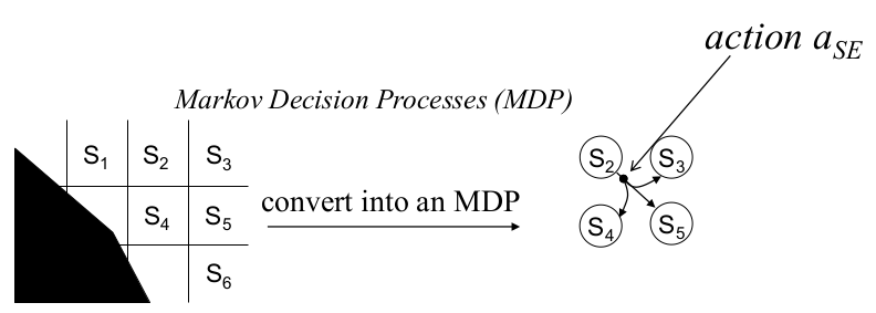
Markov Decision Processes (MDPs)

An MDP extends the deterministic planning framework by allowing each action to have multiple possible outcomes. Formally, an MDP is defined by:

• A set of states $S$
• A set of actions $A(s)$ available in each state
• For each action $a$ in state $s$:
  • a set of possible successor states
  • a probability distribution over these successors
  • an associated cost for each transition

Policy

The crucial shift when moving from deterministic planning to MDPs is that you no longer compute a single sequence of actions, since the robot may not follow the intended path. Instead, you compute a policy:

\[\pi : S \rightarrow A\]

A policy maps every state to an action — telling the robot what to do regardless of which branch of the uncertainty tree reality follows. This is why planning in MDPs is fundamentally more complex. Instead of a single path, the solution is often a directed acyclic graph (DAG) of possible transitions, representing the branching structure of all possible outcomes and the prescribed actions at each.

Objectives for Planning Under Uncertainty

In MDPs, there are multiple ways to define optimality. The lecture focuses on two:

1. Expected-cost planning: Minimize the expected total cost of reaching the goal.
2. Minimax planning: Minimize the worst-case cost, assuming the world behaves in the most adversarial possible way.

Minimax Planning

Minimax planning asks: “Given all possible uncertain outcomes, what policy minimizes the worst-case cost-to-goal?”

Formally:

\[\pi^* = \arg\min_{\pi} \max_{\text{outcomes of } \pi} {\text{cost-to-goal}}\]

In other words:

• The environment is treated as adversarial.
• The planner assumes that every action may yield the worst possible successor.
• The robot must be robust against the worst instance of randomness.

This is extremely conservative but extremely safe.

A policy maps each possible state to an action, forming a directed acyclic graph (DAG) of possible future evolutions. The graph branches wherever uncertainty exists: one action in the current state leads to multiple possible next states, each requiring its own follow-up action.

The graph contains no cycles, because in minimax reasoning a cycle would imply the robot might get stuck forever, producing infinite worst-case cost. Thus, the optimal minimax strategy is always a branching, acyclic decision structure that covers every possible outcome of uncertainty.

Computing Minimax Plans: Backward A*

Algorithm:

• Initialize $g(s_{goal}) = 0$ and $g(s) = \infty,\ \forall s \neq s_{goal}$; $OPEN = {s_{goal}}$
• while $s_{start}$ not expanded:
  • remove $s$ with smallest $f(s) = g(s) + h(s)$ from $OPEN$
  • insert $s$ into $CLOSED$
  • for every $s’$ such that $s \in succ(s’,a)$ for some $a$ and $s’$ not in $CLOSED$
    • if $g(s’) > \max_{u \in succ(s’,a)} \big(c(s’,u) + g(u) \big)$
      • $g(s’) = \max_{u \in succ(s’,a)} \big(c(s’,u) + g(u) \big)$
      • insert $s’$ into $OPEN$

After computing the minimax g-values of the states, the optimal policy is obtained by selecting an action that minimizes (think of this to be in the forward pass):

\[\text{max}_{s' \in succ(s,a)}\{c(s,a,s')+g(s')\}\]

This recursion directly encodes minimax reasoning: a state’s cost is determined by its worst possible successor, not its best or expected one.

Backward minimax A* reduces to classical backward A* when uncertainty disappears. It maintains all the properties of A* (optimality, no re-expansion) if heuristics are consistent.

Resulting Policy Structure:

The resulting minimax policy is often:

• A deterministic DAG, not a single path.
• Branching according to possible uncertain outcomes.
• Acyclic, because cycles would imply infinite worst-case cost.

The branching reflects the policy telling the robot: “If you end up in this state, take action $a$. If the uncertainty pushes you into another state, take action $b$.”

Why not Forward A*?

In deterministic planning, forward A* works beautifully because the cost of a state is determined solely by the cost accumulated so far. When you expand a state, you know exactly its future cost-to-goal because the path is deterministic. However, in minimax planning under uncertainty, every action can lead to multiple possible successor states, and the cost of a state is the maximum over the costs of all these possible outcomes.

This means that the true cost of a state cannot be known until all of its successors have been evaluated. In other words, the value of a state depends on the value of its children, not the other way around. Forward A* requires knowing or estimating the cost-to-go (the h-value) from the current state before expanding it. But in minimax, that cost is not something you can estimate from heuristics alone — it must be computed from the actual successor states. As long as those successor states are not evaluated yet, the minimax backup cannot be computed correctly.

Backward A* solves this dependency. By starting from the goal and working backward, the planner always expands states after all their successors’ values have been determined. Because the minimax backup is:

\[g(s) = \min_{a \in A(s)} \max_{u \in succ(s,a)} \big( c(s,u) + g(u) \big)\]

the value of $s$ requires knowing the values of all its successors $u$. Backward search ensures that when we compute $g(s)$, all the $g(s)$ values are already finalized or improved optimally. This maintains the same correctness and optimality guarantees that A* has in deterministic planning.

Pros and Cons of Minimax Planning

Minimax planning is powerful but expensive.

Pros:

• Extremely robust to worst-case disturbances
• Guarantees finite cost regardless of execution randomness
• Provides strong safety guarantees

Cons:

• Overly pessimistic: assumes worst-case outcome happens always
• More expensive than deterministic A*
• Heuristics are less informative because minimax backup uses max, not sum
• Backward minimax A* may not apply to all MDPs
• Even when it applies, the search is often slower because uncertainty creates branching

Thus minimax is most appropriate for safety-critical or adversarial domains where robustness outweighs efficiency.

Expected Cost Formulation

Minimax assumes that every time an action is taken, the world will produce the worst possible stochastic outcome. In many domains — navigation on slippery surfaces, noisy actuation, imperfect sensing — this assumption dramatically overestimates risk. For example, let’s say in a hill-climbing scenario, the robot has a 10% chance of slipping when moving uphill. If we treat this as an adversarial worst-case outcome, minimax will conclude that climbing is effectively impossible, because in the worst case the robot slips on every attempt. In reality, slipping occasionally is acceptable if the expected time or cost remains low.

Expected-cost planning instead models uncertainty probabilistically, so each action outcome contributes to future cost proportionally to its probability. This produces policies that are safer and more realistic than minimax, yet not overly pessimistic.

Defining the Expected-Cost Objective

The policy that is optimal under the expected-cost model minimizes:

\[\pi^* = \arg\min_{\pi} \mathbb{E}\{\text{cost-to-goal} \mid \pi\}\]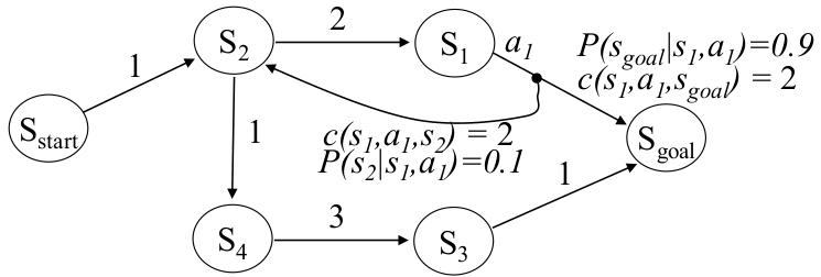

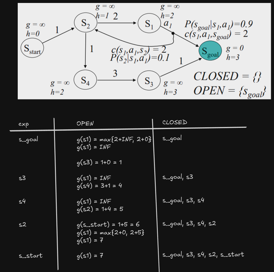
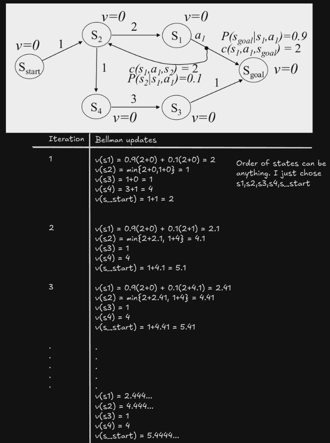
Expectation is taken over the stochastic outcomes of each action. To illustrate, consider the following example MDP:

• From $s_1$, action $a_1$ transitions
  • to $s_{goal}$ with probability $0.9$ and cost $2$
  • to $s_{2}$ with probability $0.1$ and cost $2$

Two competing strategies exist:

• $\pi_1:$ Go through $s_4$ deterministically

  Expected cost $= 1 + 1+3+1=6$

• $\pi_2:$ Keep trying to reach the goal through the stochastic $s_1$ edge

  The expected cost sums an infinite geometric series of attempts:

  \[0.9 \cdot (1+2+2)+ 0.9\cdot0.1 \cdot (1+2+2+2+2)+ 0.9\cdot0.1^2 \cdot (1+2+2+2+2+2+2) \cdots = 5.444\dots\]

Thus, under expected-cost reasoning, $\pi_2$ is better than $\pi_1$ — even though minimax preferred $\pi_1$. This highlights the fundamental philosophical difference: minimax protects against worst-case scenarios, while expected-cost planning optimizes performance on average.

Value Function

Let $v^(s)$ denote the optimal expected cost-to-goal from state $s.$ $v^(s)$ satisfies the core equation of expected-cost MDPs:

\[v^*(s) = \min_{a \in A(s)} \mathbb{E}\left[ c(s,a,s') + v^*(s') \right] \quad \text{for } s \neq s_{goal}\] \[v^*(s_{goal}) = 0\]

This is the Bellman optimality equation for stochastic shortest-path problems.

Given the optimal value function, the optimal policy is simply the greedy policy:

\[\pi^*(s) = \arg\min_{a \in A(s)} \mathbb{E}\left[c(s,a,s') + v^*(s')\right]\]

This equation formalizes the idea that an optimal action is one whose immediate cost plus expected future cost is minimal.

Value Iteration

Value Iteration solves the Bellman optimality equations through fixed-point iteration. It starts with an initial guess for all $v(s)$, then repeatedly applies the Bellman backup:

\[v(s)\leftarrow \min_{a} \mathbb{E}_{s'}\left[ c(s,a,s') + v(s') \right]\]

Important details:

• $v(s_{goal})$ is always fixed at $0$.
• It is best to initialize to admissible values (underestimates of the actual costs-to-goal).
• All other values gradually improve (monotonically increasing) until convergence.
• VI converges in a finite number of iterations. In the worst case we take $N$ sweeps, and in each sweep we take $N$ backups. So the worst case will have atmost $N^2$ backups, compared to only $N$ in A* because the order there is optimal.

• Convergence means:

  \[|v(s) - \min_{a} \mathbb{E}[c(s,a,s') + v(s')]| < \Delta\]

The order in which states are backed up affects speed but not correctness. For stochastic shortest-path problems in which every state can eventually reach the goal, VI always converges to the optimal value function.

The expected cost of executing greedy policy is at most:

\[v^*(s_{start})c_{min}/(c_{min}-\Delta)\]

VI has a drawback: it updates every state in the MDP on every iteration, even states that will never be reached by the optimal policy. This creates inefficiency in large MDPs.

Real-Time Dynamic Programming (RTDP)

While Value Iteration updates every state repeatedly, RTDP focuses computation only on states that actually matter for the optimal policy. Instead of sweeping through the entire state space, RTDP simulates execution and updates only the states encountered along greedy trajectories.

RTDP proceeds as follows:

1. Initialize all values to admissible (optimistic) underestimates.
2. Starting from the real initial state, follow a greedy policy (choosing the action that minimizes expected cost) picking outcomes at random.

3. At each visited state, apply a Bellman backup.

   \[v(s)\leftarrow \min_{a} \mathbb{E}_{s'}\left[ c(s,a,s') + v(s') \right]\]
4. If the goal is reached, restart from the start and repeat.
5. Stop when Bellman errors along the greedy path fall below $\Delta$

For the first step:

• For any state $s$, pick an action $a$ that minimizes

  \[E\{c(s,a,s')+v(s')\}\]

• Pick a successor $s’$ at random according to probability

  \[P(s'|a,s)\]

RTDP is guaranteed to converge in a finite number of iterations (given admissible initial values and a reachable goal), and like VI, it leads to an optimal greedy policy.

The expected cost of executing greedy policy is at most:

\[v^*(s_{start})c_{min}/(c_{min}-\Delta)\]

Rewards

The reward formulation is central whenever tasks do not terminate after reaching a goal, or when the robot continually interacts with the environment — patrolling, surveillance, balancing, manipulation, or any behavior that runs indefinitely. Instead of ending at a terminal state (like reaching a goal cell), the system keeps accruing rewards over time. Planning, therefore, must evaluate the long-term desirability of each state.

In a reward-based MDP, each transition gives the agent a reward $r(s,a,s’).$

The task becomes: Choose actions to maximize the expected total reward received over time.

Unlike the cost formulation, where lower values are better, here higher values are better. The optimal value function satisfies:

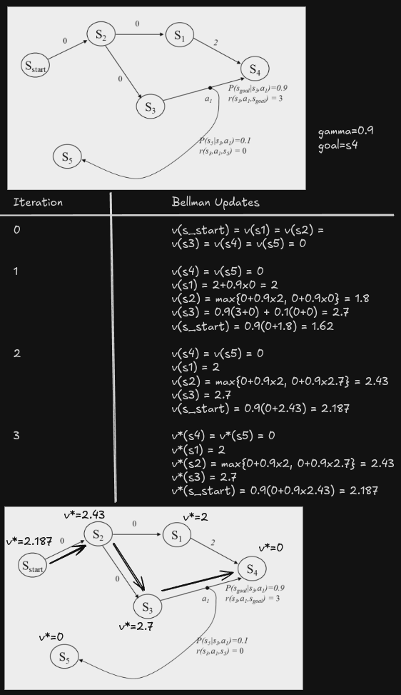
\[v^*(s) = \max_{a \in A(s)} \mathbb{E}_{s'} \big[r(s,a,s') + \gamma v^*(s') \big]\]

This is the Bellman optimality equation for reward-MDPs. The appearance of the discount factor $\gamma$ is crucial — without it, the sum of rewards could diverge, and the value function would be undefined.

Why discounting?

Discounting adjusts how the robot values immediate rewards relative to future ones:

\[0 < \gamma \le 1\]

If $\gamma \le 1:$

• Future rewards count less than immediate rewards
• Values remain finite, even if the system never terminates
• VI and PI converge rapidly, because the Bellman operator becomes a contraction

If $\gamma=1:$

• Rewards are not discounted
• Value iteration may not converge
• Total reward can become infinite if the robot loops through positive-reward cycles

Thus discounting is not merely a mathematical trick — it enforces stability and convergence in infinite-horizon tasks.

Difference in Problem Structure

In cost-based MDPs:

• There is always a terminal goal with $v^*(goal)=0$
• All states eventually must reach the goal for the formulation to be valid
• Value iteration converges because costs accumulate positively

In reward-based MDPs:

• There may be no terminal goal
• The robot may remain in the system forever (e.g., balancing a pole)
• Discounting controls infinite reward accumulation
• Policies are evaluated by their stationary, long-term behavior

The reward formulation is therefore strictly more general.

Bellman Equations Now Maximize, Not Minimize

The Bellman backup in the reward formulation becomes:

\[v(s) \leftarrow \max_{a} \mathbb{E}_{s'} \big[ r(s,a,s') + \gamma v(s') \big]\]

Compare this to the cost version:

\[v(s) \leftarrow \min_{a} \mathbb{E}_{s'} \big[ c(s,a,s') + v(s') \big]\]

The structure is the same — min becomes max, cost becomes reward, and discounting appears in the infinite-horizon setting. But the planning intuition changes dramatically: instead of trying to reach a goal cheaply, the robot tries to accumulate as much positive reward as possible.

Given the optimal value function, the optimal policy is simply the greedy policy:

\[\pi^*(s) = \arg\max_{a \in A(s)} \mathbb{E}\left[r(s,a,s') + \gamma v^*(s')\right]\]

Value Iteration for Reward MDPs

Value iteration still works — but with slightly modified behavior:

1. Initialize all values (optimistic or arbitrary).
2. Apply Bellman backups using maximization and discounting.

3. Values converge to the unique fixed point of the Bellman operator:

   \[v(s) = \max_a \mathbb{E}[ r + \gamma v(s') ]\]

Because $\gamma <1,$ the operator is a contraction — guaranteed to converge.

Partially Observable Markov Decision Processes (POMDP)

A simple path-planning example highlights the differences. In a classical graph search problem, the robot knows its exact state and every action deterministically leads to a single successor. A graph is essentially the tuple {S, A, C}: states, actions, and deterministic costs.

Once we allow action uncertainty (e.g., a drone drifting left or right with probability 0.5), the problem becomes an MDP because the effect of an action is no longer deterministic. The transition model must specify a probability over successor states:

\[T(s,a,s') = P(s' \mid s,a)\]

However, even in an MDP, the robot still assumes perfect localization: it always knows which state it lands in after acting.

In a POMDP, we remove this assumption. The robot now has uncertain state and uncertain action outcomes. It only receives limited observations that do not uniquely identify the true state. This situation arises in many robotics settings, such as UAVs navigating without GPS, mobile robots in ambiguous hallways, underwater robots with drifting odometry, or manipulation tasks where object identity is uncertain.

Thus,

• Graphs model perfect knowledge + deterministic actions.
• MDPs model full observability + stochastic actions.
• POMDPs generalize both by allowing stochastic actions and partial state observability.

What is POMDP?

A POMDP is defined as:

\[{S,\ A,\ T,\ R,\ \Omega,\ O}\]

where:

• $S:$ set of all possible world states
• $A:$ set of all actions
• $T(s,a,s’):$ transition model
• $R(s,a):$ reward (or cost) function
• $\Omega:$ set of possible observations
• $O(s’,a,o) = P(o|s’,a):$ probability of seeing observation $o$ after taking action $a$ and landing in $s’$

The critical new component is the observation model. The robot only perceives partial information about the true state.

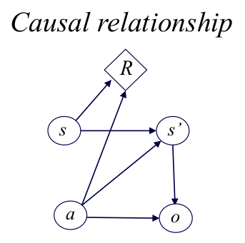
A POMDP has the following causality chain:

\[s \xrightarrow{a} s' \xrightarrow{o} \text{observation}\]

The observation does not reveal $s’$ exactly, but it narrows down possible states.