Deep Learning - Attention & Transformers

Attention Models

Problem with vanilla Seq2Seq Models

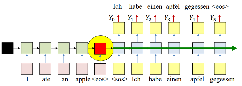
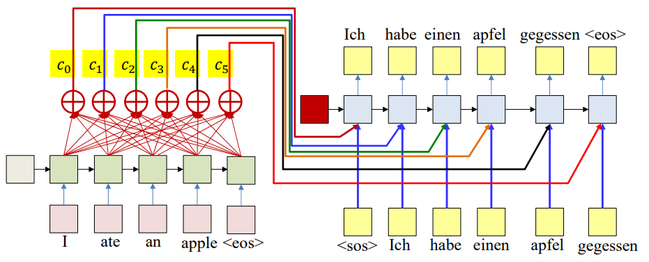
In the vanilla sequence-to-sequence (Seq2Seq) model with an encoder–decoder setup:

• The encoder reads the entire input sequence (e.g., I ate an apple) and compresses all information into a single fixed-length vector (the final hidden state).
• The decoder then uses this single vector to generate the entire output sequence (e.g., Ich habe einen Apfel gegessen).

Why is this a problem?

1. Bottleneck at the final hidden state
   • All the input information is forced into the last encoder hidden state (red box in the image above).
   • This creates an information bottleneck, especially for long sentences.
2. Decoder only gets the encoder hidden state once
   • At time step 0, the decoder receives the encoder’s final hidden state.
   • After that, the decoder only relies on its own recurrent updates, carrying forward information from previous steps.
3. Information dilution
   • As decoding progresses, the hidden state is increasingly dominated by the decoder’s own recurrence.
   • The contribution from the encoder’s final hidden state becomes weaker and “diluted.”
   • At later steps, the decoder may lose track of crucial information from the input sequence.

Because of this, for long and complex sentences, the translations or predictions degrade in quality. Moreover, important words from the beginning of the sentence may be forgotten when generating later outputs. Fundamentally, the model is assuming that a single compressed summary of the entire input is sufficient — which is not true for natural language, where each output word often depends on a specific part of the input.

Potential Solution 1

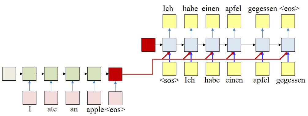
A simple solution is to have the same encoder representation feed directly into all decoder states as input. Now the decoder’s recurrence is local, and the encoder signal isn’t washed out as we move forward.

Why a single encoder vector is still not enough

Even with that change, we are still squeezing the entire input into one vector. That single vector becomes overloaded, especially for long inputs. In reality, all encoder hidden states carry information, with each one tied to its corresponding input token plus surrounding context. By relying on a single compressed summary, we inevitably lose detail, and some information from earlier tokens has already been attenuated by the time the encoder reaches its final state.

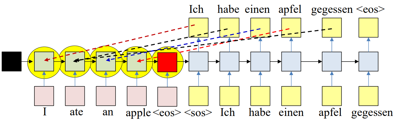
What the decoder really needs

Every output token is related to the input directly. Giving the decoder only one fixed encoder vector (even at all steps) misses the more granular relationship between individual outputs and specific parts of the input. The decoder should be able to draw, at each step, on the set of encoder states rather than only on a single summary, so it can use the portions of the input that are most relevant to the current output token.

Potential Solution 2

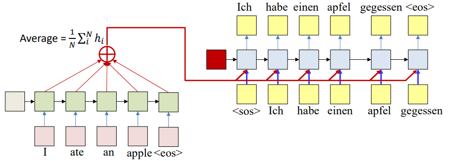
A simple approach is to compute the average of all encoder hidden states:

\[\text{Average} = \frac{1}{N} \sum_{i=1}^{N} h_i\]

This average vector is then given to the decoder at every step. This way, the decoder receives a representation that reflects the entire sequence, not just the final hidden state.

Limitations of simple averaging

While better than relying on one state, averaging has a clear drawback:

• It applies the same weight to every encoder state. Every decoder step receives the same averaged vector, regardless of which output word is being generated.
• In reality, different outputs depend on different parts of the input. For example: “Ich” is most closely related to “I”, while “habe” and “gegessen” are more related to “ate”.

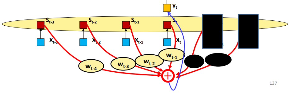
Towards Weighted Averages

The solution is to let each decoder step compute its own weighted average of the encoder hidden states.

\[c_t = \frac{1}{N} \sum_{i=1}^{N} w_i(t) h_i\]

$c_t$ is the context vector at decoding step $t$.

$w_i(t)$ are the attention weights and are dynamically computed as functions of the decoder state. The expectation is that if this model is well-trained, this will automatically highlight the correct inputs.

Attention Weights

Requirements

The attention weights depend on the decoder’s current needs. At time step $t$, they are computed using the decoder’s state from the previous step $s_{t-1}$:

\[w_i(t) = a(h_i, s_{t-1})\]

where $a(.)$ is a function (called the alignment model or score function) that measures how well encoder state $h_i$ matches the decoder state $s_{t-1}$.

For the system to work properly, the attention weights must satisfy two conditions:

1. Each weight must be positive

2. All weights for step $t$ must sum to $1$, forming a probability distribution

   \[\sum_{i=1}^{N} w_i(t) = 1\]

To meet these requirements, we compute weights in two stages:

1. Compute a set of raw scores that can be positive or negative

   \[e_i(t) = g(h_i, s_{t-1})\]

   where $g$ is the scoring function.

2. Convert these scores into valid weights using the softmax function

   \[w_i(t) = \frac{\exp(e_i(t))}{\sum_j \exp(e_j(t))}\]

This guarantees that $w_i(t) \ge 0, \space \sum_i w_i(t) = 1.$

Options for scoring function:

1. Dot Product Attention

\[g(h_i, s_{t-1}) = h_i^T s_{t-1}\]

1. General Attention

   \[g(h_i, s_{t-1}) = h_i^T W_g s_{t-1}\]

   $W_g$ needs to be learned.

2. Concat (Additive) Attention

   \[g(h_i, s_{t-1}) = v_g^T \tanh ( W_g \begin{bmatrix} h_i \\ s_{t-1}\end{bmatrix} \big)\]

   $v_g, W_g$ need to be learned.

3. MLP-based Attention

   \[g(h_i, s_{t-1}) = \text{MLP}([h_i, s_{t-1}])\]

   $\text{MLP}$ needs to be learned.

We will be using the general attention scoring function.

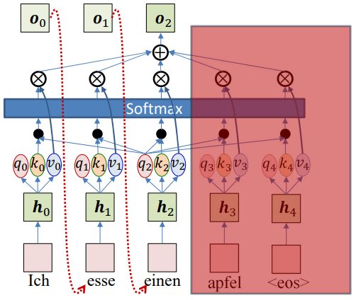
Query-Key-Value

Query–Key–Value (QKV) introduces a more flexible and general framework:

• Each input is represented by a key and a value.
• Keys represent how an input is searched or matched. Values represent the actual content/information to be passed.
• Each decoder step generates a query. Queries represent what the decoder is currently looking for.
• Attention weights are computed as a function of query and keys, and the final context is a weighted sum of values.

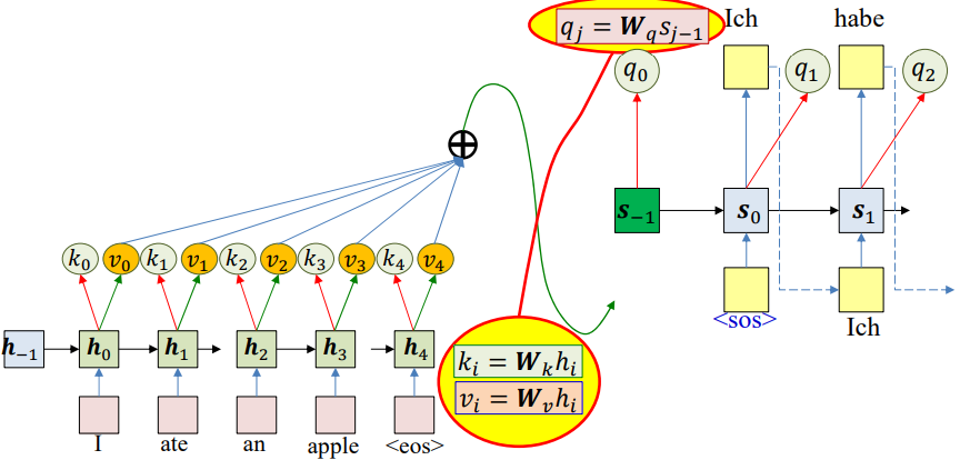
Keys and values are derived from encoder hidden states:

\[k_i = W_kh_i\] \[v_i = W_vh_i\]

Query is derived from the decoder state:

\[q_t = W_qs_{t-1}\]

Attention weights are computed as a function of query and keys:

\[e_i(t) = g(k_i,q_t)\] \[w_i(t) = softmax(e_i(t))\]

Context is a weighted sum of values:

\[c_i(t) = \sum_iw_i(t)v_i\]

Pseudocode:

# Assuming encoded input is available
# (K,V) = [k_enc[0], k_enc[1], ..., k_enc[T]], [v_enc[0], v_enc[1], ..., v_enc[T]]

t = -1
h_out[-1] = 0   # Initial Decoder hidden state
q[0] = 0        # Initial query 

Y_out[0] = <sos>
do 
	t = t+1
	C = compute_context_with_attention(q[t], K, V)
	y[t],h_out[t],q[t+1] = RNN_decode_step(h_out[t-1], y_out[t-1], C)
	y_out[t] = generate(y[t]) # Random, or greedy
until y_out[t] == <eos>

function compute_context_with_attention(q, K, V)
	# First compute attention
	e = []
	for t = 1:T # Length of input
	e[t] = raw_attention(q, K[t])
	end
	maxe = max(e) # subtract max(e) from everything to prevent underflow
	a[1..T] = exp(e[1..T] - maxe) # Component-wise exponentiation
	suma = sum(a) # Add all elements of a
	a[1..T] = a[1..T]/suma
	
	C = 0
	for t = 1..T
		C += a[t] * V[t]
	end
	
	return C

Beam Search

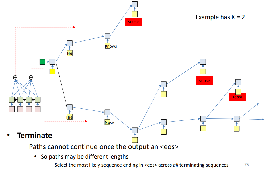
Our general goal is to generate the most likely output sequence that ends with <eos>. If we simply pick the most likely word at each step (greedy decoding), it can lead to suboptimal sequences. Example: Choosing “Ich → habe → einen → apfel” step-by-step may fail if another slightly less probable choice early on leads to a better overall translation.

So, instead of committing to just one choice at each step, we retain multiple candidate paths. Each word choice forks the network, creating parallel hypotheses. This allows the model to explore different continuations of the sequence.

However, keeping all possible continuations would be computationally infeasible. So we prune by keeping only the top K most likely candidate sequences at each time step,

Process:

• At each step, compute the probability of partial sequences:

  \[P(O_1, O_2, \ldots, O_t \mid I_1, I_2, \ldots, I_N)\]
• Retain the Top-K scoring sequences (based on the product of probabilities)
• Continue extending them until <eos> is reached

Different paths may reach <eos> at different lengths. The final output will be the likely complete sequence ending in <eos>.

Pseudocode:

# Assuming encoder output H = hin[1]… hin[T] is available
path = <sos>
beam = {path}
pathscore = [path] = 1
state[path] = h[0] # computed using your favorite method
context[path] = compute_context_with_attention(h[0], H)
do # Step forward
	nextbeam = {}
	nextpathscore = []
	nextstate = {}
	nextcontext = {}
	for path in beam:
		cfin = path[end] 
		hpath = state[path]
		C = context[path]
		y,h = RNN_decode_step(hpath, cfin, C)
		nextC = compute_context_with_attention(h, H)
		for c in Symbolset
			newpath = path + c
			nextstate[newpath] = h
			nextcontext[newpath] = nextC
			nextpathscore[newpath] = pathscore[path]*y[c]
			nextbeam += newpath # Set addition
		end
	end
	beam, pathscore, state, context, bestpath = prune (nextstate, nextpathscore, nextbeam, nextcontext)
until bestpath[end] = <eos>

Training

• In the forward pass, the encoder reads the input sentence and produces a sequence of hidden states that capture contextual meaning of each word.
• At each step, the decoder looks at its own previous hidden state, the last generated word, and a context vector formed by attention over encoder states. This gives a probability distribution over possible next words in the target language.
• Once we have the predicted distributions, we compare them with the actual ground truth sequence.
• We compute the divergence, and this loss is then backpropagated through the decoder, attention module, and encoder, so that every parameter learns to adjust in a way that improves translation accuracy next time.

However, if we always feed the predicted word into the next decoder hidden state, the early training predictions will be poor because these is no one-to-one correspondence between the input and the ouput. So instead, since we already know the target or the true next word, we feed that in directly. This is called teacher forcing, and it makes training much easier because the decoder always has the right context, and the model converges faster.

The problem with pure teacher forcing is that at inference time, the decoder won’t have access to ground truth, and its own mistakes can snowball (a mismatch called exposure bias). So instead, we find the middle ground where sometimes we feed the ground truth, and sometimes feed the predicted word. We could even gradually shift from more teacher forcing early on to less later in training.

Another trick is sampling from the model’s predicted distribution instead of always taking the most likely word. This makes training closer to inference, because at inference we don’t have ground truth and the model must rely on its own probabilities. But sampling is not naturally differentiable (you can’t backpropagate through the act of choosing one word). To solve this, we use the Gumbel-Softmax trick.

Gumbel Noise Trick:

The Gumbel trick allows differentiable sampling.

1. Given decoder logits $l_i$, we add Gumbel noise $g_i$:

   \[z_i = l_i + g_i, \quad g_i \sim \text{Gumbel(0,1)}\]
   • This transforms logits into a set of noisy scores.
   • The max of these corresponds to a true categorical sample.

2. Instead of taking a hard max, apply a softmax with temperature $\tau$:

   \[y_i = \frac{\exp(z_i / \tau)}{\sum_j \exp(z_j / \tau)}\]
   • $y$ is now a continuous vector, approximating a one-hot sample.
   • As $\tau \rightarrow 0:$ output becomes nearly one-hot
   • As $\tau \rightarrow \inf:$ output becomes uniform
   • High $\tau$ implies soft & exploratory, low $\tau$ implies sharp & close to true sampling

Multi-Head Attention

Instead of a single attention function, we use multiple sets of projections of keys, queries, and values.

\[k_i^l = W_k^l h_i, \quad v_i^l = W_v^l h_i, \quad q_j^l = W_q^l s_{j-1}\]

• $l$ is the head index
• Each head has its own learnable $W_k^l, W_v^l, W_q^l$

So for each head:

• It computes its own attention scores $e_i^l(t)$
• Produces its own context vector $c_t^l$

After all heads compute their contexts, we concatenate and project them:

\[\text{MultiHead}(Q,K,V) = W_o \big[ c_t^1 ; c_t^2 ; \dots ; c_t^h \big]\]

Purpose of Multi-Head:

• Each head learns to focus on different aspects of the input.
  • One head might align with word position.
  • Another might capture semantic meaning.
  • Another might handle long-range dependencies.
• Improves representation power by letting the model look at the same sequence from different subspaces.

Self-Attention

Problem with Recurrent Encoders

• In standard encoder-decoder models with RNNs, each hidden state $h_i$ is computed sequentially and contains information from all previous words.
• When the decoder attends to these $h_i$ vectors, it is implicitly attending to the entire sequence again, not just the specific word.
• This raises a question: If the decoder is already selecting relevant words through attention, do we really need recurrence in the encoder at all?

Instead of using recurrence, we can directly compute embeddings for all words in parallel:

\[h_i = f(x_i)\]

where $f$ could be a simple MLP applied to the word embedding $x_i$.

But this removes the context-specificity:

• Example: the word “an” may map to “ein”, “einer”, or “eines” in German depending on context.
• Purely local embeddings $h_i$ lose this adaptability.

So the solution is to use the attention framework itself to introduce contextspecificity in embeddings.

Self-Attention

• Use the attention mechanism itself to inject context into embeddings.
• Each word’s representation is updated by attending to all other words in the sequence (including itself).
• This creates context-sensitive embeddings without recurrence.

Computing Self-Attention

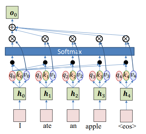
1. Initial hidden representations

   Each word gets an initial representation:

   \[h_i = f(x_i)\]

2. Compute Queries, Keys, and Values

   For each word embedding $h_i$:

   \[q_i = W_qh_i, \quad k_i=W_kh_i, \quad v_i = W_vh_i\]

   where $W_q, W_k,W_v$ are learnable matrices.

3. Attention scores

   The attention score between word $i$ and word $j$ is a function of query $q_i$ and key $k_j$:

   \[e_{ij} = q_i^Tk_j\]

4. Normalize via Softmax

   \[w_{ij} = \frac{\exp(e_{ij})}{\sum_{j=1}^N\exp(e_{ij})}\]

   This gives the attention weight of word $i$ on word $j$.

   \[w_{i0}, \ldots, w_{iN} = softmax(e_{i0}, \ldots e_{iN})\] \[w_{ij}=attn(q_i, k_{0:N})\]

5. Compute New Representation

   The updated embedding for word $i$ is:

   \[o_i = \sum_{j=1}^Nw_{ij}v_j\]

   This means each word now carries information from all other words in proportion to attention weights.

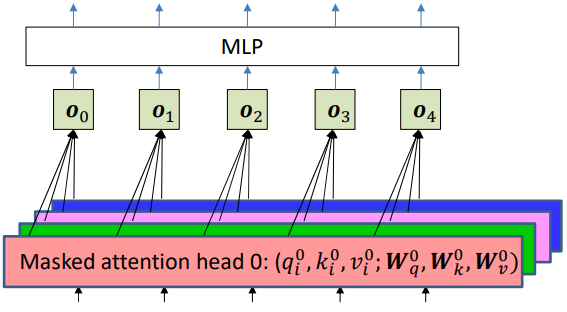
Multi-Head Self-Attention

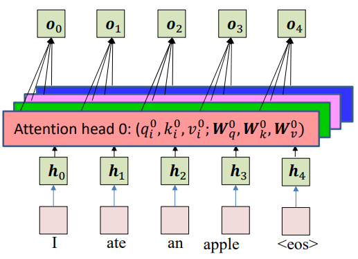
To capture different aspects of relationships simultaneously, we can also have multiple attention heads.

For each head $a$, we project hidden state $h_i$ into queries, keys, and values using learnable matrices:

\[q_i^a = W_q^a h_i \] \[k_i^a = W_k^a h_i\] \[v_i^a = W_v^a h_i\]

Each head has its own $W_q^a, W_k^a, W_v^a.$

For each head $a$, compute attention weights and outputs:

\[w_{ij}^a = \text{attn}(q_i^a, k_{0:N}^a)\] \[o_i^a = \sum_j w_{ij}^a v_j^a\]

Each head produces its own output representation $o_i^a$, and different heads focus on different aspects of the input. Once all heads compute their outputs, we concatenate them:

\[o_i = [o_i^1;o_i^2;o_i^3;\ldots;o_i^H]\]

where $H$ is the number of heads.

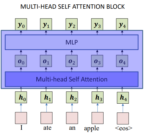
The concatenated vector is passed through an MLP (feedforward block):

\[y_i = \text{MLP}(o_i)\]

Typically, this is a linear transformation + nonlinearity (ReLU/GeLU), and helps mix the information across heads.

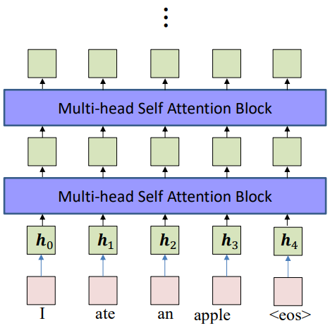
The encoder can include many layers of suck multi-head self-attention blocks, and there is no need for recurrence.

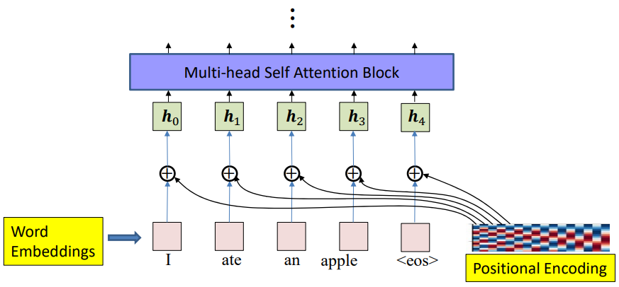
Positional Encoding

Need to know relative position

Attention mechanisms treat the input sequence as a set of tokens without inherent order. Unlike RNNs or CNNs, there is no built-in sense of sequence or distance between words. But in language, relative position matters:

• “dog bites man” ≠ “man bites dog”
• Words closer together often influence each other more strongly than words far apart.

Without positional information, self-attention compares every token with every other token equally — the attention score between tokens does not depend on their relative distance. For example, the influence of “an” on “apple” should be much stronger when they are adjacent, and weaker when separated by many words.

Thus, we add positional encodings to word embeddings to inject sequence order into the model, giving the network awareness of word positions and distances.

Properties:

We define a sequence of vectors $P_t$ for each position $t$. These vectors have the following properties:

1. Each position has a unique encoding:

   \[P_{t_1} \neq P_{t_2}, \quad \text{for } \space t_1 \neq t_2\] \[|P_t|^2 = C\]

2. The correlation between two position encodings falls off with distance:

   \[|P_t \cdot P_{t+\tau_1}| > |P_t \cdot P_{t+\tau_2}|, \quad \text{if } |\tau_1| < |\tau_2|\]

3. The correlation is stationary, meaning it depends only on the distance, not the absolute positions:

   \[P_{t_1} \cdot P_{t_1+\tau} = P_{t_2} \cdot P_{t_2+\tau}\]

Constructing Positional Encodings:

The most widely used approach (from the original Transformer paper) is to use sinusoids of different frequencies. For a token at position $t$ and embedding dimension $d$:

\[P_t = \begin{bmatrix} \sin(\omega_1 t) \\ \cos(\omega_1 t) \\ \sin(\omega_2 t) \\ \cos(\omega_2 t) \\ \vdots \\ \sin(\omega_{d/2} t) \\ \cos(\omega_{d/2} t) \end{bmatrix}\] \[\omega_l = \frac{1}{10000^{2l/d}}, \quad l = 1, \dots, d/2\]

Thus, even and odd dimensions alternate between sine and cosine functions at exponentially decreasing frequencies.

\[P_t[2i] = \sin \left( \omega_i t \right), \quad P_t[2i+1] = \cos \left( \omega_i t \right)\]

The encoding preserves relative distances. For any position $t$ and offset $\tau$:

\[P_{t+\tau} = M_\tau P_t\]

where

\[M_\tau = \text{diag} \left( \begin{bmatrix} \cos(\omega_l \tau) & \sin(\omega_l \tau) \\ -\sin(\omega_l \tau) & \cos(\omega_l \tau) \end{bmatrix}, \quad l = 1 \dots d/2 \right)\]

This means the positional encoding shifts in a predictable way when moving from one position to another, allowing the model to learn shift-invariant (translation-invariant) relationships.

So now, with positional encoding, we have a mechanism where the attention that we pay to a word also depends on how far away it is.

Masked Self-Attention

The idea of removing recurrence using self-attention can be extended to the decoder as well. However, in the decoder, generation is sequential. At step $t$, we only know outputs up to $t$ (previous words). So we must prevent looking ahead at future tokens.

This is done by masking: when computing attention weights, we set $e_{ij} = -\inf$ if $j>i.$ This forces the softmax to ignore future words.

\[w_{ij} = \begin{cases} \frac{\exp(e_{ij})}{\sum_{m=1}^i \exp(e_{im})}, & j \leq i \\ 0, & j > i \end{cases}\]

And the output is still:

\[o_i = \sum_{j=1}^i w_{ij} v_j\]

This is called masked self-attention, ensuring that each word prediction depends only on past outputs.

Just like in the encoder, we stack multiple masked self-attention layers followed by feedforward layers (MLPs).

A block looks like:

1. Masked self-attention
2. Feedforward MLP with nonlinearity (e.g., ReLU)
3. Residual connections + normalization

Masked Mullti-Head Self-Attention

Instead of a single set of $Q,K,V,$ we use multiple heads, just like we did before:

\[q_i^a = W_q^a h_i, \quad k_i^a = W_k^a h_i, \quad v_i^a = W_v^a h_i\]

Each head computes its own weighted sum:

\[o_i^a = \sum_{j=1}^i w_{ij}^a v_j^a\]

The outputs of all heads are concatenated:

\[o_i = [o_i^1; o_i^2; \dots; o_i^H]\]

This allows different heads to capture different aspects of dependencies (e.g., short-range vs. long-range).

We can also add positional encoding, like we did for the encoders.

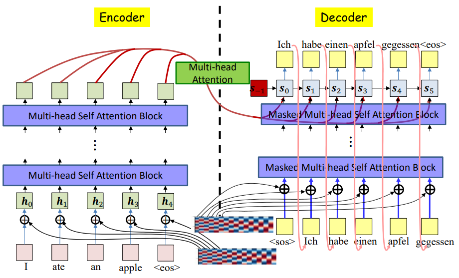
Transformers

Architecture

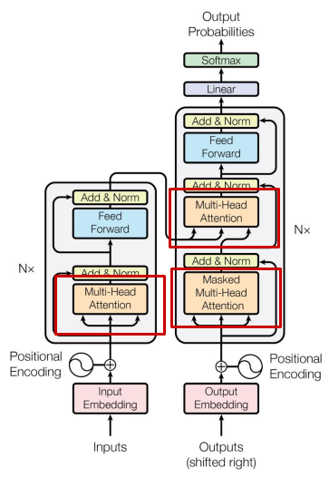
Components:

1. Tokenization – Convert text into discrete tokens
2. Embedding Layer – Map tokens into continuous vectors
3. Self-Attention (Multi-Headed) – Compute contextual representations
4. Position Encoding – Add word order information
5. Feed-Forward Network (FFN) – Apply non-linear transformations
6. Residual Connections + Layer Normalization – Stabilize and improve training
7. Output Projection Layer – Map to vocabulary logits

Tokenization

• Splits text into smaller units (words, subwords, characters).
• Each token is represented by an index in the vocabulary.

Example: The sentence “CMU’s 11785 is the best deep learning course” becomes token IDs [3, 5, 100, 57, ..., 1].

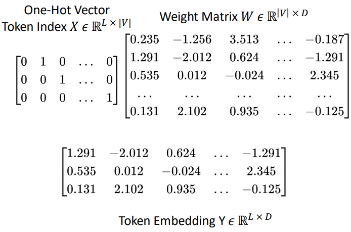
Embeddings

Converts discrete token IDs into dense vectors using an embedding matrix. In Pytorch, it is the function nn.Embedding, and is essentially a linear layer.

If vocabulary size $

V

$, embedding dimension $D$, and sequence length $L$, then:

\[X ∈ ℝ^{L × |V|}, \quad W ∈ ℝ^{|V| × D}\] \[Y = XW, \quad Y ∈ ℝ^{L × D}\]

$X$ is the one-hot vector, $W$ is the weight matrix, and $Y$ is the token embedding.

So, each token index is mapped to a continuous embedding vector.

Self-Attention

For input $X \in ℝ^{L×D}$:

\[Q = XW_Q, \quad K = XW_K, \quad V = XW_V\]

where $W_Q, W_K, W_V \in ℝ^{D×d_k}$.

Compute similarity between queries and keys:

\[e_{ij} = \frac{Q_i \cdot K_j^T}{\sqrt{d_k}}\] \[w_{ij} = softmax(e_{ij})\] \[O_i = \sum_j w_{ij} V_j\]

Multi-Head Attention

• Instead of one attention map, use multiple heads.
• Each head projects Q, K, V differently, capturing diverse relationships.
• Outputs are concatenated:

\[MHA(Q,K,V) = Concat(head_1, ..., head_h)W_O\]

Attention Masking

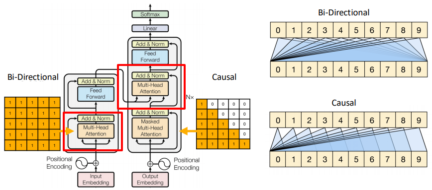
• Bidirectional attention (encoder): Each token attends to all tokens.
• Causal attention (decoder): Masks future tokens to prevent cheating during training.

Cross-Attention

• Used in encoder-decoder models.
• Decoder queries come from previous outputs, keys and values come from encoder outputs.

We do not need to mask in cross-attention because the encoder sequence is fully known from the start.

• The input sentence (source) is fixed and complete.
• There’s no notion of “future” tokens in the source — every encoder hidden state can be used freely.
• So when the decoder attends to the encoder, it’s fine to use all encoder tokens.

Masking is only needed where there’s autoregressive generation (decoder self-attention), not when attending to a fully known sequence (encoder outputs).

Positional Encoding

Since attention is permutation-invariant, we add positional encodings to capture order.

\[p_t^{(i)} = f(t)^{(i)} := \begin{cases} \sin(\omega_k \cdot t), & \text{if } i = 2k \\ \cos(\omega_k \cdot t), & \text{if } i = 2k+1 \end{cases} \quad \text{where} \quad \omega_k = \frac{1}{10000^{2k/d}}\]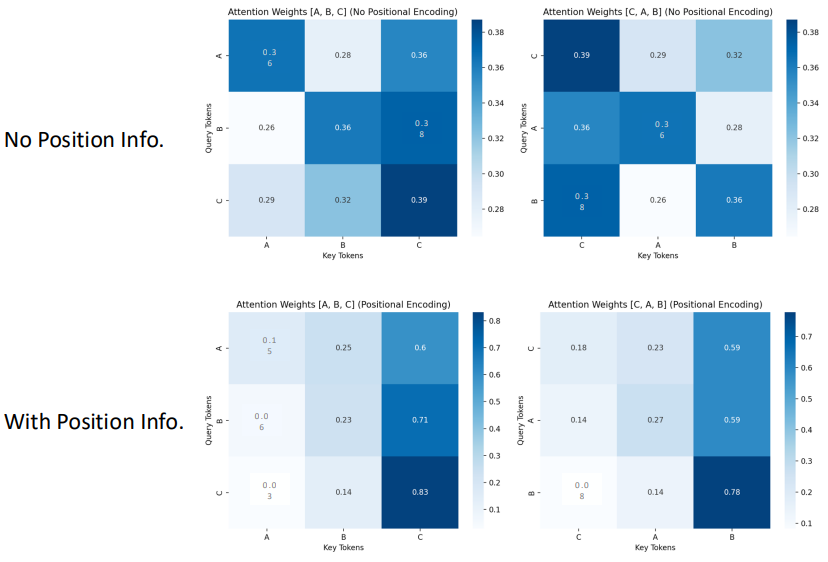

Feed-Forward Block

A two-layer MLP applied to each position independently.

\[FFN(x) = \max(0, xW_1 + b_1)W_2 + b_2\]

Residual Connections & Layer Normalization

Residual connections, also called skip connections, allow each block to learn a refinement over its input instead of learning a transformation from scratch.

\[x_{t+1} = x_t + F(x_t)\]

where $F(x_t)$ is the function of the block (like Multi-Head Attention or Feed-Forward Network).

This prevents vanishing gradients and allows information to flow directly across layers.

Normalization stabilizes training by scaling inputs to have mean 0 and variance 1. In Layer Norm, the normalization is applied across the embedding dimension of each token and each token vector is normalized independently:

\[\text{LN}(h) = \frac{h - \mu}{\sigma} \cdot \gamma + \beta\]

The position of LayerNorm relative to the residual connection changes training dynamics.

1. Post-Norm (original Transformer)

   • Apply residual connection first, then normalize:

     \[x_{t+1} = \text{LN}(x_t + F(x_t))\]
   • Pros: empirically achieves slightly higher performance when tuned well.
   • Cons: harder to train, gradients may explode/vanish for deep models.
2. Pre-Norm (modern variants, e.g., GPT-2, BERT)

   • Normalize input before applying the block function:

     \[x_{t+1} = x_t + F(\text{LN}(x_t))\]
   • Pros: much more stable and easier to train, especially for very deep networks.
   • Cons: may cap performance a bit if not tuned, but usually negligible.

Improvements on Transformers

Types of Architectures

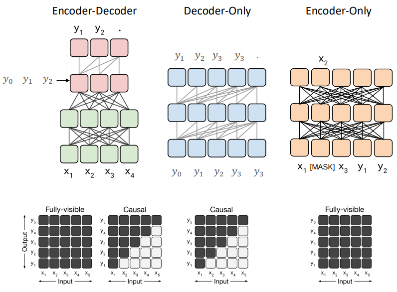
Encoder-Decoder:

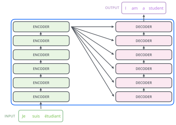
• Same design as in the original Transformer paper.
• Input (prompt or source text) goes into the encoder.
• The decoder generates the output sequence step by step, attending both to previous outputs (masked self-attention) and encoder outputs (cross-attention).
• Used for tasks that map one text to another (translation, summarization, etc.).

Encoder-Only (BERT):

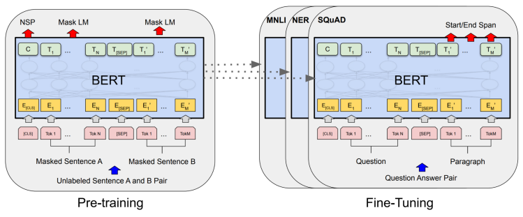
• Uses only the encoder stack.
• Training objectives:
  • Masked Language Modeling (MLM): randomly mask tokens and predict them.
  • Next Sentence Prediction (NSP): predict if two sentences follow each other.
• Produces contextualized representations of tokens that can be fine-tuned for downstream tasks (classification, QA, etc.).

Decoder-Only (GPT):

• Uses only the decoder stack with causal masking.
• Trained with next token prediction (standard language modeling).
• Naturally suited for text generation tasks.

Positional Encoding

Absolute Position Encoding:

\[PE_{(t, 2i)} = \sin\left(\frac{t}{10000^{2i/d}}\right) \ PE_{(t, 2i+1)} = \cos\left(\frac{t}{10000^{2i/d}}\right)\]

Relative Position Encoding:

Instead of encoding absolute index, encode relative distance between tokens.

Attention score modification:

\[e_{ij} = \frac{q_i \cdot k_j}{\sqrt{d}} + b_{i-j}\]

where $b_{i-j}$ is a learnable bias depending on relative distance.

The advantage of this is that it has better generalization to longer sequences than trained on.

Rotary Position Encoding (RoPE):

• Standard sinusoidal positional encodings (used in original Transformers) add position information to token embeddings.
• RoPE instead represents position by rotating embeddings in a 2D plane.
• This technique is used in modern LLMs such as LLaMA.
• Advantage: Encodes relative positions naturally and improves generalization to longer contexts.

Each query and key vector is multiplied by a complex exponential to encode its position:

• Rotation in 2D space corresponds to multiplying by $e^{i\theta}$
• Thus, embeddings are rotated depending on their sequence position.

For a query token at position $m$ and a key at position $n$:

\[f_q(x_m, m) = (W_q x_m) e^{i m \theta}\] \[f_k(x_n, n) = (W_k x_n) e^{i n \theta}\]

The dot product (attention score) between them is:

\[g(x_m, x_n, m-n) = \text{Re}\Big[ f_q(x_m, m) \cdot f_k(x_n, n)^* \Big]\] \[g(x_m, x_n, m-n) = \text{Re} \left[ (W_q x_m)(W_k x_n)^{*} e^{i (m-n)\theta} \right]\]

The exponential factor $e^{i(m-n)\theta}$ encodes the relative distance between positions $m,n$. This allows the model to directly incorporate relative positional information into attention scores.

Instead of using complex numbers, RoPE can be expressed as a rotation matrix applied to even–odd index pairs of the embedding vector:

\[f_{q,k}(x_m, m) = R^d_{\Theta, m} W_{q,k} x_m\] \[R^d_{\Theta, m} = \begin{bmatrix} \cos(m\theta_1) & -\sin(m\theta_1) & & & & \\ \sin(m\theta_1) & \cos(m\theta_1) & & & & \\ & & \cos(m\theta_2) & -\sin(m\theta_2) & & \\ & & \sin(m\theta_2) & \cos(m\theta_2) & & \\ & & & & \ddots & \\ & & & & & \cos(m\theta_{d/2}) & -\sin(m\theta_{d/2}) \\ & & & & & \sin(m\theta_{d/2}) & \cos(m\theta_{d/2}) \end{bmatrix}\]

Each pair of dimensions undergoes a rotation by an angle proportional to $m\theta_j$.

Efficient Attention Mechanism

The vanilla self-attention mechanism has quadratic time and memory complexity with respect to sequence length $L.$

\[Attention(Q, K, V) = softmax\left(\frac{QK^T}{\sqrt{d_k}}\right)V\]

This requires:

• Time complexity: $O(L^2d)$ FLOPs
• Memory complexity: $O(L^2)$

For long sequences (e.g., 4k–32k tokens), this quadratic cost becomes a major bottleneck.

Linear Attention:

Idea: Replace the softmax with a kernel function that allows factorization.

Standard softmax attention:

\[\text{Softmax}(QK^T)V = \frac{\exp(QK^T)}{\sum_{i=1}^L \exp(QK_i^T)}V\]

Instead, approximate similarity using a kernel function $\phi(.):$

\[\text{sim}(Q,K) = \phi(Q)\phi(K)^T\]

Thus attention becomes linearized:

\[\frac{\phi(Q)\phi(K)^T}{\sum_{i=1}^L \phi(Q)\phi(K_i)^T}V = \frac{\phi(Q) (\phi(K)^TV)}{\phi(Q)\sum_{i=1}^L\phi(K_i)^T}\]

Complexity drops from $O(L^2)$ to $O(Ld’^2)$.

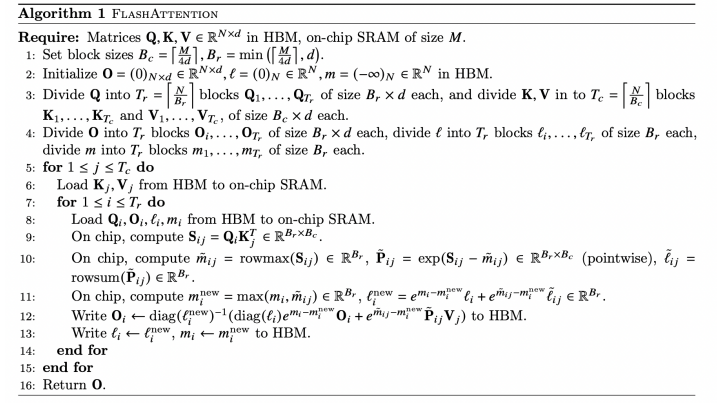
Flash Attention:

Standard attention stores the huge $L \times L$ matrix in memory. Flash Attention avoids materializing it. Instead it computes attention block by block, directly in GPU high-bandwidth memory (HBM).

The trick is to:

• Fuse operations into a single GPU kernel (matrix multiplication + softmax + scaling).
• Use tiling: split matrices into small blocks that fit into SRAM.
• Reduces memory reads/writes by orders of magnitude.

Issues with softmax:

• Naive Softmax requires 2 loops:
  1. Compute normalizer $\sum_je^{x_j}$
  2. Divide each exponential
• Safe Softmax adds a max-subtraction step for numerical stability.

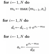
• Online Softmax combines steps to reduce passes.

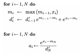
Flash Attention fuses this into one loop:

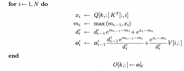
This keeps the normalization stable without ever storing the full matrix.

IO complexity:

• Standard attention: $\Omega(Nd+N^2)$
• Flash attention: $O(\frac{N^2d^2}{M})$, where $M$ is SRAM size

This results in e-3x speedup and ~10x less memory usage.

KV Caching:

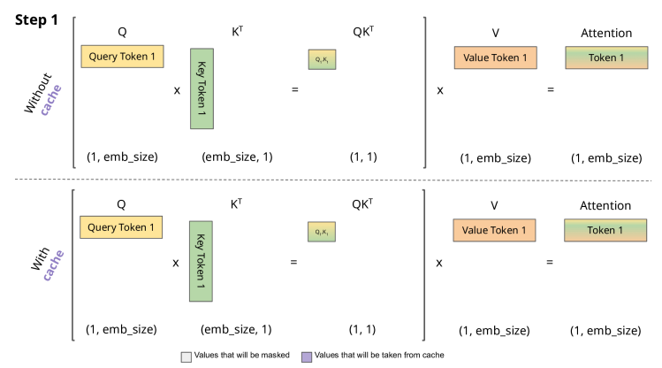
When decoding autoregressively (LLMs), recomputing all past $K,V$ at each step is wasteful.

So the trick is to:

• Cache previously computed Key and Value vectors.
• For the next token, only compute new $K_t,V_t$ and append to cache.

This avoids recomputation, reducing complexity per token from $O(L^2)$ to $O(L)$.

Multi and Grouped Query Attention:

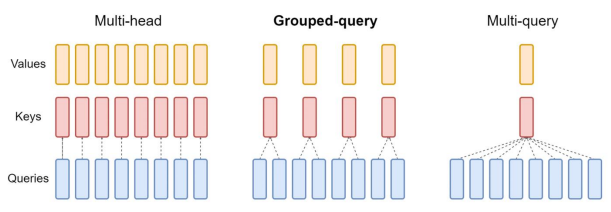
Standard Multi-head Attention (MHA):

• In normal multi-head attention, we have H independent sets of queries, keys, and values.
• This means memory + compute cost grows with H.

Multi-query Attention (MQA):

• Shares the same keys and values across all query heads.
• Only queries are separate per head.
• This reduces memory cost, since we only store one set of K and V, instead of H.

Grouped-query Attention (GQA):

• A middle ground between MHA and MQA.
• Queries are divided into groups, where each group shares a single key and value set.
• Reduces KV memory footprint more than MHA but not as aggressively as MQA.
• Better accuracy than MQA since it doesn’t collapse all queries into one KV set.

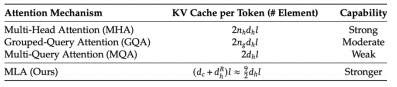
Multi-Head Latent Attention:

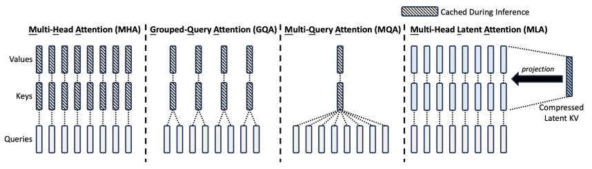
MLA improves on MQA/GQA by:

• Low-rank compression of K and V: Instead of directly caching K and V, MLA projects them into a latent space.
• Stores compressed latent representations (much smaller).
• During inference, only compressed KV pairs are cached, reducing memory usage while maintaining accuracy.

Parameter Efficient Tuning

Traditional fine-tuning involves updating all parameters of a large pre-trained transformer for each downstream task. However, this is expensive in memory and compute.

Parameter Efficient Tuning methods update only a small proportion of parameters, while keeping most of the pre-trained model frozen.

Prefix Tuning:

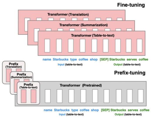
• Idea: Learn a small set of continuous prefix vectors (virtual tokens) that are prepended to the input at each layer.
• The transformer parameters remain frozen; only these prefix vectors are trained.
• Works well for sequence generation tasks (translation, summarization, table-to-text).

Prompt Tuning:

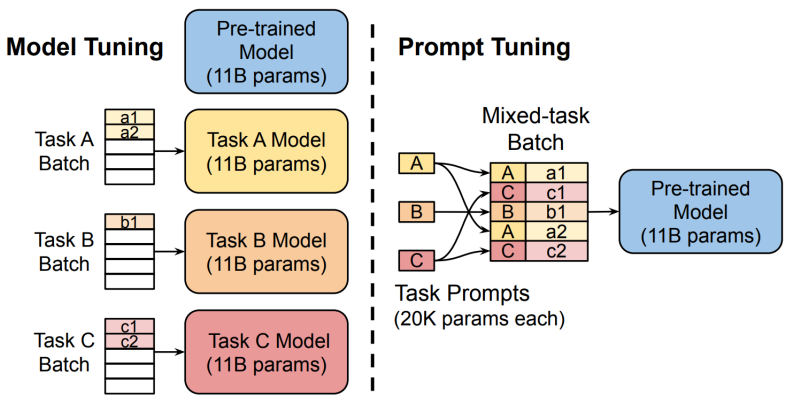
• Similar to prefix tuning but even lighter: Learns a small set of soft prompt embeddings (tokens) specific to each task.
• Instead of modifying all layers, only the input embedding space is modified.
• Allows a single pre-trained model to adapt to many tasks by swapping task-specific prompts.

Adapter:

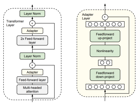
• Introduce small MLP “adapter” layers inside each transformer layer (usually after feedforward or attention).
• During training, pre-trained weights stay frozen, and only adapter parameters are updated.
• Advantage: Easy to plug in; allows good transfer across tasks.

LoRA (Low-Rank Adaptation):

• Replace large weight update matrices with a low-rank decomposition.

• Instead of updating $W,$ represent update as:

  \[h = W_0 x + \Delta W x = W_0 x + B A x\]

where:

• $W_0:$ frozen pre-trained weight
• $A,B:$ small trainable low-rank matrices
• Much fewer trainable parameters