In Progress

To-Do

CNNs — all
LSTM, GRU
Connectionist Temporal Classification

Convolutional Neural Networks

https://youtu.be/kYeeB3CNcx8?si=otHbiKRITjJZk9S8

Forward Pass

# Input:
#   Y(0, :, :, :) = Image     # The input image (or feature map) is stored at layer 0
#                             # Dimensions: (channels, width, height)

# Iterate over each convolutional layer
for l = 1:L                          # L = total number of layers

    # Iterate over the spatial positions (x, y) of the output feature map
    for x = 1:(W_{l-1} - K_l + 1)    # Slide window horizontally
        for y = 1:(H_{l-1} - K_l + 1) # Slide window vertically

            # Iterate over the output channels (filters)
            for j = 1:D_l
                z(l, j, x, y) = 0     # Initialize pre-activation (accumulator)

                # Accumulate contributions from all input channels
                for i = 1:D_{l-1}        # D_{l-1} = # input channels to layer l
                    for x' = 1:K_l       # K_l = kernel width
                        for y' = 1:K_l   # K_l = kernel height

                            # Perform convolution at this location:
                            # weight * input value
                            z(l, j, x, y) += w(l, j, i, x', y') * Y(l-1, i, x + x' - 1, y + y' - 1)
                            # Note: (x + x' - 1) and (y + y' - 1) are for correct indexing

                # Apply activation function (e.g. ReLU) after convolution
                Y(l, j, x, y) = activation(z(l, j, x, y))

# Final prediction Y is obtained by flattening the last layer's output and applying softmax
Y = softmax(Y(L, :, 1, 1) .. Y(L, :, W - K + 1, H - K + 1))

Backpropagation

I don’t think I can do a better job in explaining CNN backpropagation than this video. Just watch it. But here’s the pseudo code for quick reference.

# Start with gradient of the loss w.r.t. the final layer output
dY(L) = dDiv / dY(L)    # From loss function 

# Loop backward through layers
for l = L : downto : 1                             # Backprop layer-by-layer
    dw(l) = zeros(D_l × D_{l-1} × K_l × K_l)       # Initialize weight gradient
    dY(l - 1) = zeros(D_{l-1} × W_{l-1} × H_{l-1}) # Initialize input gradient

    # Loop over spatial positions in the output feature map
    for x = W_{l-1} - K_l + 1 : downto : 1
        for y = H_{l-1} - K_l + 1 : downto : 1
            for j = D_l : downto : 1              # For each output channel

                # Backprop through activation
                dz(l, j, x, y) = dY(l, j, x, y) * f′( z(l, j, x, y) )

                # Backpropagate error and compute weight gradients
                for i = D_{l-1} : downto : 1          # Input channels
                    for x′ = K_l : downto : 1         # Kernel width
                        for y′ = K_l : downto : 1     # Kernel height

                            # Chain rule: propagate error to input
                            dY(l - 1, i, x + x′ - 1, y + y′ - 1) += \
                                w(l, j, i, x′, y′) * dz(l, j, x, y)

                            # Compute gradient of weight
                            dw(l, j, i, x′, y′) += \
                                dz(l, j, x, y) * Y(l - 1, i, x + x′ - 1, y + y′ - 1)

Recurrent Neural Networks

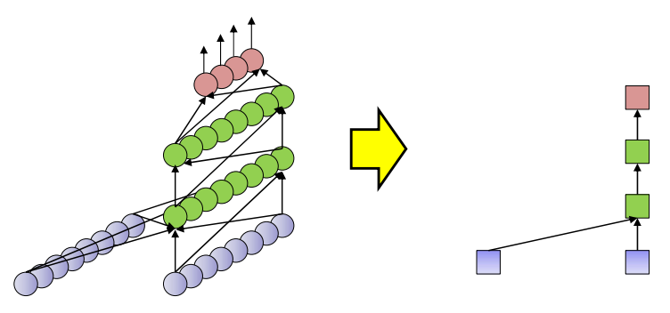
State-Space Model

State-space model is a model for infinite response systems.

\[h_t = f(x_t,h_{t-1}) \\\] \[y_t = g(h_t)\]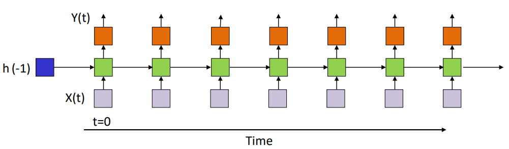

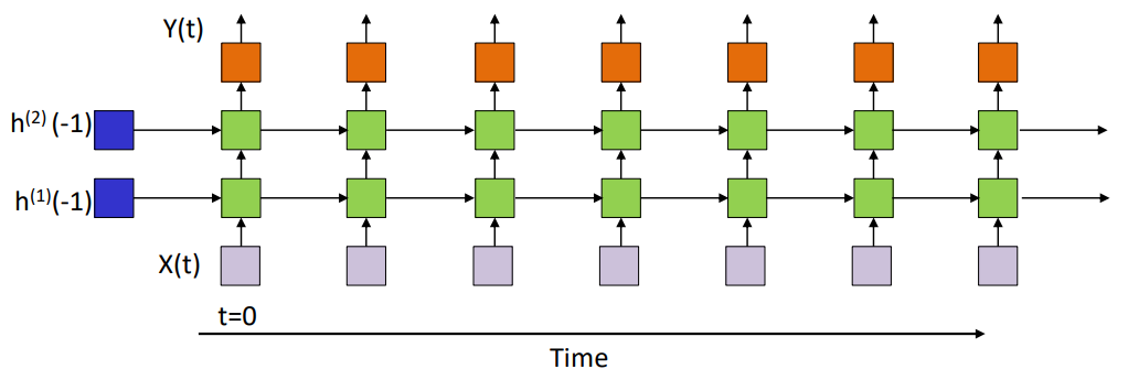
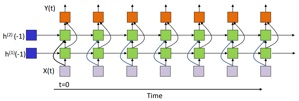
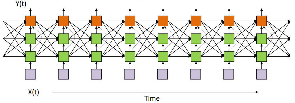
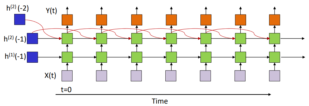
There are all different types of RNNs, having varying number of layers.

Considering an RNN with just one hidden layer,

\[h_i^{(1)}(t) = f_1 \left( \sum_j w_{ji}^{(1)} x_j(t) + \sum_j w_{ji}^{(11)} h_j^{(1)}(t-1) + b_i^{(1)} \right) \\\] \[Y_k(t) = f_2 \left( \sum_j w_{jk}^{(2)} h_j^{(1)}(t) + b_k^{(2)} \right), \quad k = 1..M\]

In the vector form:

\[\textbf{h}^{(1)}(t) = f_1(\textbf{W}^{(1)}\textbf{X}(t)+\textbf{W}^{(11)}\textbf{h}^{(1)}(t-1)+\textbf{b}^{(1)}) \\\] \[\textbf{Y}(t) = f_2(\textbf{W}^{(2)}\textbf{h}^{(1)}(t)+\textbf{b}^{(2)})\]

$f_1()$ is usually the $\tanh$ activation function.

The hidden state captures both new input and temporal memory via the recurrent connection.
Output depends only on the current hidden state, but that hidden state has a history encoded in it through $h(t-1), h(t-2),$ etc.
The initial values of hidden states are generally learnable paramteres as well.

Variants on RNNs

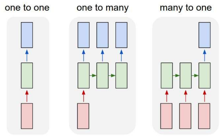
One to one: Conventional MLP
One to many: Sequence generation, e.g. image to caption
Many to one: Sequence based prediction or classification, e.g. Speech recognition, text classification
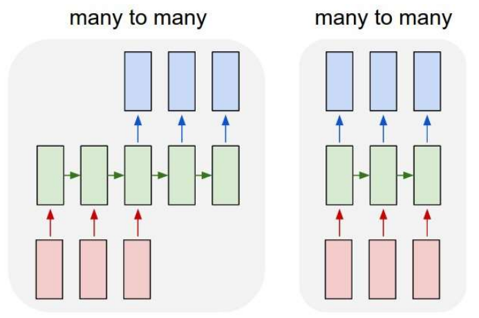
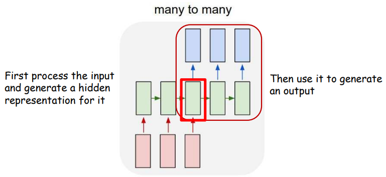
Many to many: Delayed sequence to sequence, e.g. machine translation
Many to many: Sequence to sequence, e.g. stock problem, label prediction

Training

Forward Pass

for t = 0:T-1:
	# Initialize input vectors
	h(t,0) = x(t)
	for l = 1:L:
		z(t,l) = Wc(l) * h(t,l-1) + Wr(l) * h(t-1,l) + b(l) # c for current, r for recurrent
		h(t,l) = tanh(z(t,l))
	zo(t,L) = Wo(L) * h(t,L) + bo
	Y(t) = softmax(zo(t,L))

Assuming $h(-1,^*)$ is known
Assuming $L$ hidden-state layers and an output layer
$W_c, W_r$ are matrices, $b$ are vectors
$W_c$ are weights for inputs from current time
$W_r$ are recurrent weights applied from previous time
$W_o$ are output layer weights

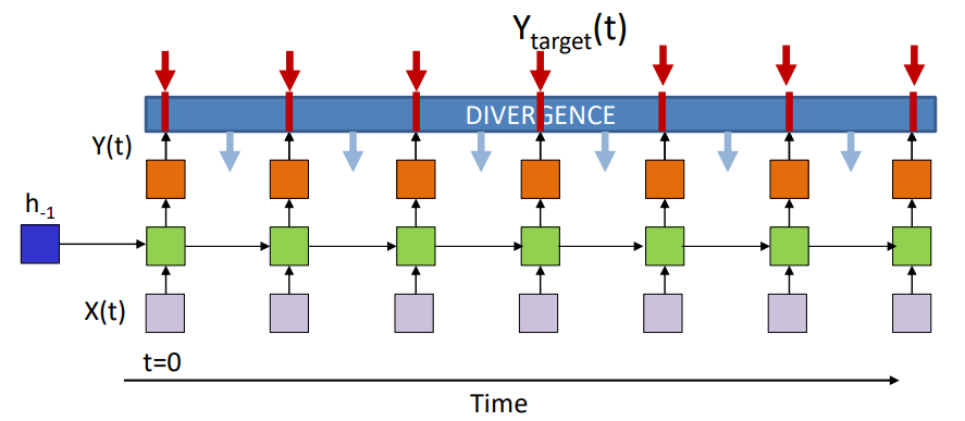
Back Propagation Through Time (BPTT)

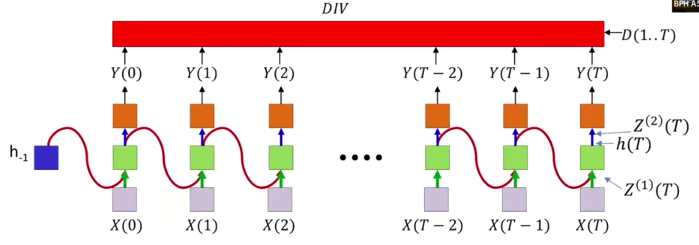
The divergence computed is between the sequence of outputs by the network and the desired sequence of outputs. So $DIV$ is a scalar function of a series of vectors.

The $DIV$ is not necessarily the sum of divergences at individual times, unless we explicitly define it to be that way.

Local Gradients from Output:

We want:

\[\frac{\partial DIV}{\partial Y_i(t)} \space \space \text{for all i,t}\]

If $DIV$ is the sum of all divergences, then

\[\frac{\partial DIV}{\partial Y_i(t)} = \frac{\partial Div(t)}{\partial Y_i(t)}\]

In any case, let’s assume we know how to compute this gradient. We will tackle what exact divergence helps us do this later.

Backprop for the last time sequence:

Final layer
\[\nabla_{Z^{(2)}(T)} DIV = \nabla_{Y(T)} DIV \cdot \nabla_{Z^{(2)}(T)} Y(T)\]
For element-wise output activation:
\[\frac{dDIV}{dZ_i^{(2)}(T)} = \frac{dDIV}{dY_i(T)} \cdot \frac{dY_i(T)}{dZ_i^{(2)}(T)}\]
For vector output activation:
\[\frac{dDIV}{dZ_i^{(2)}(T)} = \sum_j \frac{dDIV}{dY_j(T)} \cdot \frac{dY_j(T)}{dZ_i^{(2)}(T)}\]
For final layer weights
\[\nabla_{W^{(2)}} DIV = h(T) \nabla_{Z^{(2)}(T)} DIV\] \[\frac{dDIV}{dw_{ij}^{(2)}} = \frac{dDIV}{dZ_j^{(2)}(T)} \cdot h_i(T)\]
To hidden state
\[\nabla_{h(T)} DIV = \nabla_{Z^{(2)}(T)} DIV \cdot W^{(2)}\] \[\frac{dDIV}{d h_i(T)} = \sum_j \frac{dDIV}{dZ_j^{(2)}(T)} \cdot \frac{dZ_j^{(2)}(T)}{d h_i(T)} = \sum_j w_{ij}^{(2)} \cdot \frac{dDIV}{dZ_j^{(2)}(T)}\]

\[\nabla_{Z^{(1)}(T)} DIV = \nabla_{h(T)} DIV \cdot \nabla_{Z^{(1)}(T)} h(T)\] \[\frac{dDIV}{dZ_i^{(1)}(T)} = \frac{dDIV}{dh_i(T)} \cdot \frac{dh_i(T)}{dZ_i^{(1)}(T)}\]

Weights to hidden state
\[\nabla_{W^{(1)}} DIV = X(T) \cdot \nabla_{Z^{(1)}(T)} DIV\] \[\frac{dDIV}{dw_{ij}^{(1)}} = \frac{dDIV}{dZ_j^{(1)}(T)} \cdot X_i(T)\] \[\nabla_{W^{(11)}} DIV = h(T - 1) \cdot \nabla_{Z^{(1)}(T)} DIV\] \[\frac{dDIV}{dw_{ij}^{(11)}} = \frac{dDIV}{dZ_j^{(1)}(T)} \cdot h_i(T - 1)\]

Progressing backward in time:

Final layer
\[\nabla_{Z^{(2)}(T-1)} DIV = \nabla_{Y(T-1)} DIV \cdot \nabla_{Z^{(2)}(T-1)} Y(T-1)\] \[\frac{dDIV}{dZ_i^{(2)}(T-1)} = \frac{dDIV}{dY_i(T-1)} \cdot \frac{dY_i(T-1)}{dZ_i^{(2)}(T-1)}\] \[\frac{dDIV}{dZ_i^{(2)}(T-1)} = \sum_j \frac{dDIV}{dY_j(T-1)} \cdot \frac{dY_j(T-1)}{dZ_i^{(2)}(T-1)}\]
For final layer weights
\[\frac{dDIV}{dw_{ij}^{(2)}} += \frac{dDIV}{dZ_j^{(2)}(T-1)} \cdot h_i(T-1)\] \[\nabla_{W^{(2)}} DIV += h(T-1) \cdot \nabla_{Z^{(2)}(T-1)} DIV\]
Since the RNN uses the same weights at each time step (weight sharing), the total gradient of the loss with respect to $\textbf{W}^{(2)}$ is the sum of the gradients over all time steps. Hence we have the increment
To hidden state
\[\nabla_{h(T-1)} DIV = \nabla_{Z^{(2)}(T-1)} DIV \cdot W^{(2)} + \nabla_{Z^{(1)}(T)} DIV \cdot W^{(11)}\] \[\frac{dDIV}{d h_i(T-1)} = \sum_j w_{ij}^{(2)} \frac{dDIV}{d Z_j^{(2)}(T-1)} + \sum_j w_{ij}^{(11)} \frac{dDIV}{d Z_j^{(1)}(T)}\] \[\nabla_{Z^{(1)}(T-1)} DIV = \nabla_{h(T-1)} DIV \cdot \nabla_{Z^{(1)}(T-1)} h(T-1)\] \[\frac{dDIV}{d Z_i^{(1)}(T-1)} = \frac{dDIV}{d h_i(T-1)} \cdot \frac{d h_i(T-1)}{d Z_i^{(1)}(T-1)}\]
Weights to hidden state
\[\nabla_{W^{(1)}} DIV \mathrel{+}= X(T-1) \cdot \nabla_{Z^{(1)}(T-1)} DIV\] \[\frac{dDIV}{dw_{ij}^{(1)}} \mathrel{+}= \frac{dDIV}{dZ_j^{(1)}(T-1)} \cdot X_i(T-1)\] \[\nabla_{W^{(11)}} DIV \mathrel{+}= h(T-2) \cdot \nabla_{Z^{(1)}(T-1)} DIV\] \[\frac{dDIV}{dw_{ij}^{(11)}} \mathrel{+}= \frac{dDIV}{dZ_j^{(1)}(T-1)} \cdot h_i(T-2)\]

We continue this until

\[\nabla_{h_{-1}} DIV = \nabla_{Z^{(1)}(0)} DIV \cdot W^{(11)}\] \[\frac{dDIV}{dh_i(-1)} = \sum_j w_{ij}^{(11)} \cdot \frac{dDIV}{dZ_j^{(1)}(0)}\]

# Assuming forward pass has been completed
# Jacobian(x, y) is the Jacobian of x w.r.t. y
# Assuming dY(t) = ∇_{Y(t)}DIV is available for all t
# Assuming all dZ, dH, dW and db are initialized to 0

for t = T-1 : downto : 0
    # ∇_{Z^{(2)}(t)}DIV = ∇_{Y(t)}DIV × ∇_{Z^{(2)}(t)}Y(t)
    dZ_o(t) = dY(t) × Jacobian(Y(t), Z_o(t))  

    # ∇_{W^{(2)}}DIV += h(t, L)^T × ∇_{Z^{(2)}(t)}DIV
    dW_o += h(t, L)ᵀ × dZ_o(t)

    # db_o += ∇_{Z^{(2)}(t)}DIV
    db_o += dZ_o(t)

    # ∇_{h(t, L)}DIV += ∇_{Z^{(2)}(t)}DIV × W^{(2)}
    dH(t, L) += dZ_o(t) × W_oᵀ

    # --- Reverse through layers ---
    for l = L : downto : 1
        # ∇_{Z^{(1)}(t,l)}DIV = ∇_{h(t,l)}DIV × ∇_{Z^{(1)}(t,l)}h(t,l)
        dZ(t, l) = dH(t, l) × Jacobian(h(t, l), Z(t, l))

        # ∇_{h(t,l-1)}DIV += ∇_{Z^{(1)}(t,l)}DIV × W_c(l)
        dH(t, l-1) += dZ(t, l) × W_c(l)

        # ∇_{h(t-1,l)}DIV += ∇_{Z^{(1)}(t,l)}DIV × W_r(l)
        dH(t-1, l) += dZ(t, l) × W_r(l)

        # ∇_{W_c(l)}DIV += h(t,l-1)^T × ∇_{Z^{(1)}(t,l)}DIV
        dW_c(l) += h(t, l-1)ᵀ × dZ(t, l)

        # ∇_{W_r(l)}DIV += h(t-1,l)^T × ∇_{Z^{(1)}(t,l)}DIV
        dW_r(l) += h(t-1, l)ᵀ × dZ(t, l)

        # ∇_{b(l)}DIV += ∇_{Z^{(1)}(t,l)}DIV
        db(l) += dZ(t, l)

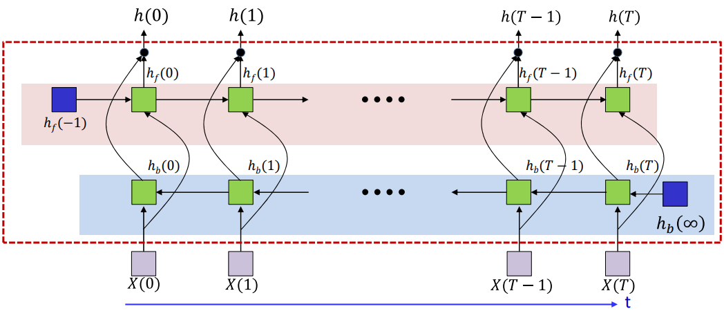
Bidirectional RNN

Inference

# Subscript "f" → forward RNN, subscript "b" → backward RNN
# x(t) is input sequence at time t (could be output from a lower layer)
# Assume h_f(-1,*) and h_b(∞,*) are known initializations

# --- Forward recurrence (left to right in time) ---
for t = 0 : T-1                         # Looping forward through time
    h_f(t, 0) = x(t)                    # Input to first layer (layer 0)
    for l = 1 : L_f                     # L_f is depth of forward RNN
        # z_f(t,l) = W_fc × h_f(t, l-1) + W_fr × h_f(t-1, l) + b_f
        z_f(t, l) = W_fc(l) × h_f(t, l-1) + W_fr(l) × h_f(t-1, l) + b_f(l)

        # h_f(t,l) = tanh(z_f(t,l))      # Assuming tanh activation
        h_f(t, l) = tanh(z_f(t, l))

# --- Backward recurrence (right to left in time) ---
h_b(T, :, :) = h_b(∞, :, :)             # Initial hidden state for backward pass
for t = T-1 : downto : 0                # Looping backward through time
    h_b(t, 0) = x(t)                    # Input to first layer (layer 0)
    for l = 1 : L_b                     # L_b is depth of backward RNN
        # z_b(t,l) = W_bc × h_b(t, l-1) + W_br × h_b(t+1, l) + b_b
        z_b(t, l) = W_bc(l) × h_b(t, l-1) + W_br(l) × h_b(t+1, l) + b_b(l)

        # h_b(t,l) = tanh(z_b(t,l))
        h_b(t, l) = tanh(z_b(t, l))

# --- Output from bidirectional layer ---
for t = 0 : T-1
    # Concatenate forward and backward hidden states at final layer
    h(t) = [h_f(t, L_f); h_b(t, L_b)]

Forward Pass

# Inputs:
#   L     : Number of hidden layers
#   Wc    : Current weights of each layer (input-to-hidden)
#   Wr    : Recurrent weights of each layer (hidden-to-hidden)
#   b     : Biases for each layer
#   hinit : Initial hidden state (e.g., h(-1,*))
#   x     : Input vector sequence [T x input_dim]
#   T     : Length of the input sequence
#
# Output:
#   h     : Hidden activations after tanh
#   z     : Pre-activations (linear sums before tanh)

function RNN_forward(L, Wc, Wr, b, hinit, x, T)
    h(-1,:) = hinit                  # h(-1) = hinit for all layers

    for t = 0:T-1                    # Forward through time
        h(t,0) = x(t)                # Input goes into "layer 0"
        for l = 1:L                 # Forward through layers
            # Linear sum: zᶫₜ = Wc(l) * h(t, l-1) + Wr(l) * h(t-1, l) + b(l)
            z(t,l) = Wc(l) * h(t,l-1) + Wr(l) * h(t-1,l) + b(l)
            
            # Non-linearity: hᶫₜ = tanh(zᶫₜ)
            h(t,l) = tanh(z(t,l))   
        end
    end

    return h

# Subscript "f" = forward net
# Subscript "b" = backward net
# Assuming:
#   h_f(-1, :) is known as initial state
#   h_b(∞, :) is known as terminal state

# Forward pass: go left-to-right
h_f = RNN_forward(Lf, Wfc, Wfr, b_f, h_f(-1,:), x, T)

# Backward pass: go right-to-left
x_rev = fliplr(x)                   # Flip input in time
h_brev = RNN_forward(Lb, Wbc, Wbr, b_b, h_b(inf,:), x_rev, T)
h_b = fliplr(h_brev)                # Flip hidden sequence to match forward time

# Combine both forward and backward outputs for each time step:
for t = 0:T-1
    # Final output h(t) is a concat of last layer forward + backward
    h(t) = [h_f(t, Lf); h_b(t, Lb)]
    # You can also use another output layer like: y(t) = W_o * h(t)
end

Back Propagation Through Time

# Inputs:
#   L       : Number of hidden layers
#   W_c, W_r, b : current (feedforward) weights, recurrent weights, and biases
#   hinit   : Initial hidden state (corresponds to h(-1,*))
#   x       : Input sequence (T time steps)
#   T       : Length of input sequence
#   dh_top  : Gradient from the layer above (dDIV/dh(t,L) for all t)
#   h, z    : Stored values from the forward pass

# Output:
#   dx      : Gradient w.r.t input x(t)
#   dW_c    : Gradient w.r.t current weights
#   dW_r    : Gradient w.r.t recurrent weights
#   db      : Gradient w.r.t bias
#   dh(-1)  : Gradient w.r.t initial hidden state

function RNN_bptt(L, W_c, W_r, b, hinit, x, T, dh_top, h, z)
    dh = zeros                  # initialize full dh(t,l)
    
    for t = T-1:down to:0      # Backward through time
        dh(t, L) += dh_top(t)  # Add top gradient to dh(t, L)
        h(t, 0) = x(t)         # Initialize input to first layer
        
        for l = L:1            # Reverse through layers
            dz(t,l) = dh(t,l) * Jacobian(h(t,l), z(t,l))     # ∇h → ∇z using chain rule
            dh(t, l-1) += dz(t,l) * W_c(l)                   # Backprop through current weights
            dh(t-1, l) = dz(t,l) * W_r(l)                    # Backprop through recurrent weights

            dW_c(l) += h(t, l-1) * dz(t,l)                   # Accumulate ∂L/∂W_c
            dW_r(l) += h(t-1, l) * dz(t,l)                   # Accumulate ∂L/∂W_r
            db(l)   += dz(t,l)                               # Accumulate ∂L/∂b
        dx(t) = dh(t,0)                                      # Gradient w.r.t. input x(t)

    return dx, dW_c, dW_r, db, dh(-1)  # dh(-1) = dh(-1,1:L,:) → for use by previous layer

# Assumptions:
#   dh(t)     : Gradient from the upper layer, shape (T, Lf+Lb)
#   x(t)      : Input to the BRNN block
#   z_f, h_f  : Forward net activations (t=0...T-1)
#   z_b, h_b  : Backward net activations (t=0...T-1)
#   Lf, Lb    : Number of forward and backward layers

for t = 0:T-1
    dh_f(t) = dh(t, 1:Lf)              # Split forward part
    dh_b(t) = dh(t, Lf+1:Lf+Lb)        # Split backward part

# === Forward Net Backprop ===
[dx_f, dW_fc, dW_fr, db_f, dh_f(-1)] = 
    RNN_bptt(L, W_fc, W_fr, b_f, h_f(-1,:), x, T, dh_f, h_f, z_f)

# === Backward Net Backprop ===
x_rev = fliplr(x)                      # Reverse input time order
dh_brev = fliplr(dh_b)                 # Reverse dh_b
h_brev = fliplr(h_b)                   # Reverse activations
z_brev = fliplr(z_b)                   # Reverse preactivations

[dx_brev, dW_bc, dW_br, db_b, dh_b(inf)] = 
    RNN_bptt(L, W_bc, W_br, b_b, h_b(inf,:), x_rev, T, dh_brev, h_brev, z_brev)

dx_b = fliplr(dx_brev)                # Flip back the dx

# === Combine the gradients from both passes ===
for t = 0:T-1
    dx(t) = dx_f(t) + dx_b(t)         # Total gradient w.r.t input x(t)

Behavior of Recurrence

BIBO Stability

Time-delay structures have bounded input if:

The activation function $f()$ has a bounded output for a bounded input, and this is generally the case for every activaton function that we use
The input $X(t)$ is bounded

This is called the “Bounded Input Bounded Output” stability, and is highly desirable.

Is a Recurrent Network BIBO?

If a non-linear activation is used, then the output obtained from it is always bounded and hence behaves as a BIBO.

But what if we use a linear activation function? To understand this, we can analyze only the behavior of the recurrent hidden layer $h_t$. This is called the Streetlight effect. Consider the following example of an identity activation:

\[z_t = W_hh_{t-1} + W_xx_t \\ h_t = z_t\]

Now,

\[h_t = W_hh_{t-1} + W_xx_t \\ h_{t-1} = W_hh_{t-2} + W_xx_{t-1}\]

This gives,

\[h_t = W_h^2h_{t-2} + W_hW_xx_{t-1} + W_xx_t\]

Repeating this for the entire time series, we get,

\[h_t = W_h^{t+1}h_{-1} + W_h^tW_xx_0 + W_h^{t-1}W_xx_1 + W_h^{t-2}W_xx_2 + \ldots + W_xx_t\]

This becomes,

\[h_t = H_t(h_{-1}) + H_t(x_0) + H_t(x_1) + ... H_t(x_t)\]

If $H_t(x_0)$ blows up, the entire system blows up. If this does not blow up, then the responses to later inputs will also not blow up.

So $h_k$ is a sum of weighted transformations of all past inputs and the initial state.

Suppose we have nothing else except the input $x(0)$.

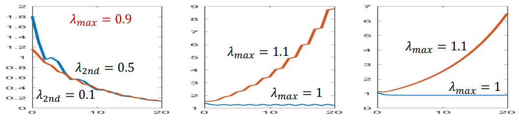
\[h_0(t) = W^t C x(0)\]

So the response at time $t$ is governed by the matrix power $W^t$. Assume $W$ is diagonalisable. Then the power of $W$ is

\[W^t = U \Lambda^t U^{-1}\]

with

\[\Lambda^t = \begin{bmatrix}\lambda_1^t & 0 & 0 \\0 & \lambda_2^t & 0 \\0 & 0 & \ddots\end{bmatrix}\]

Lets say $\lambda_1$ is the largest eigenvalue of $W.$ Then by bringing it outside the matrix, we have

\[\Lambda^t = \lambda_1^t\begin{bmatrix}1 & 0 & 0 \\0 & (\frac{\lambda_2}{\lambda_1})^t & 0 \\0 & 0 & \ddots\end{bmatrix}\]

So this essentially becomes dominated by the largest eigenvalue $\lambda_1$.

\[h_0(t) = W^t C x(0) = U \Lambda^t U^{-1} C x(0)\]

The growth or decay of $h(t)$ as $t \rightarrow \inf$ is controlled by the largest eigenvalue of $W$:

If $|\lambda_1| > 1, h(t)$ grows exponentially — system blows up
If $|\lambda_1| < 1, h(t)$ shrinks to zero — system vanishes
If $|\lambda_1| = 1, h(t)$ is marginally stable
Complex eigenvalues will cause oscillatory reponse but with the same overall trends

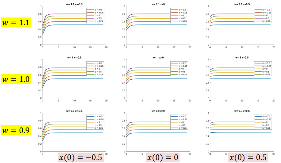
With a non-linear activation function:

Sigmoid
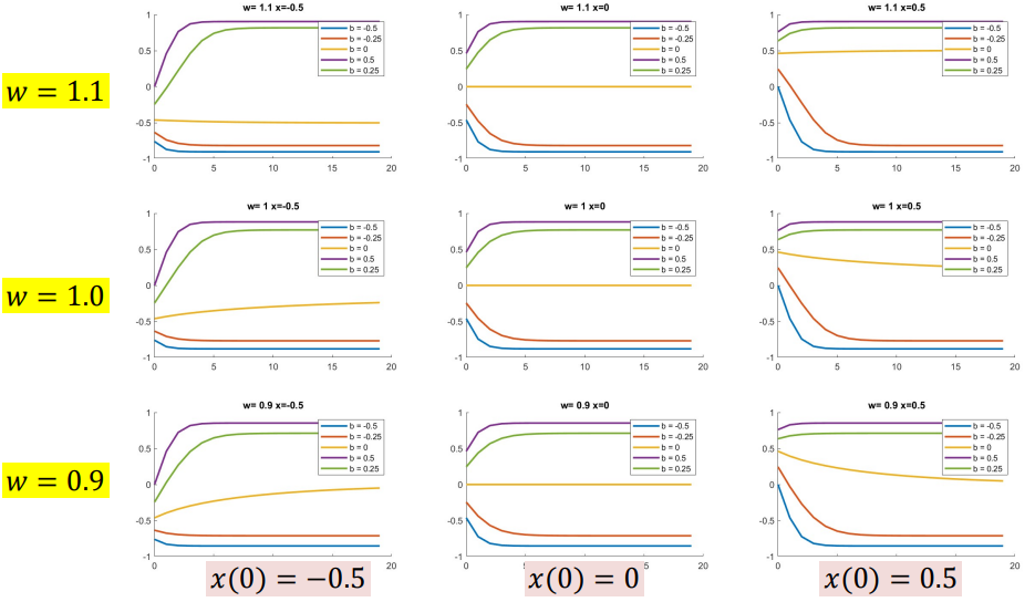
\[h(t) = sigmoid(wh(t-1) +cx(t)+b)\]
Final value depends only on $b, w$ and not $x$
Tanh
\[h(t) = tanh(wh(t-1) +cx(t)+b)\]
Final value depends only on $b, w$ and not $x$
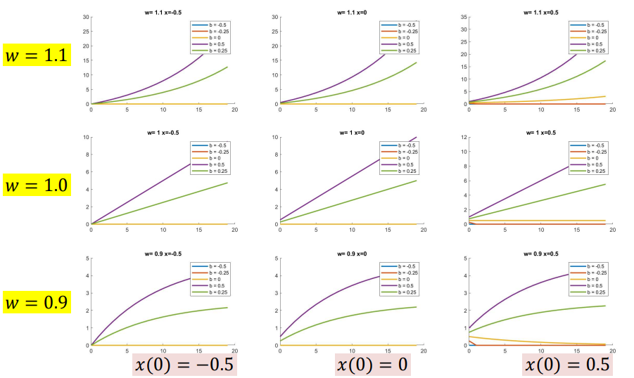
ReLU
\[h(t) = relu(wh(t-1) +cx(t)+b)\]
Relu blows up if $w>1$ for $x>0$, and dies for $x<0$. So it is pretty unstable and useless

For a vector processing:

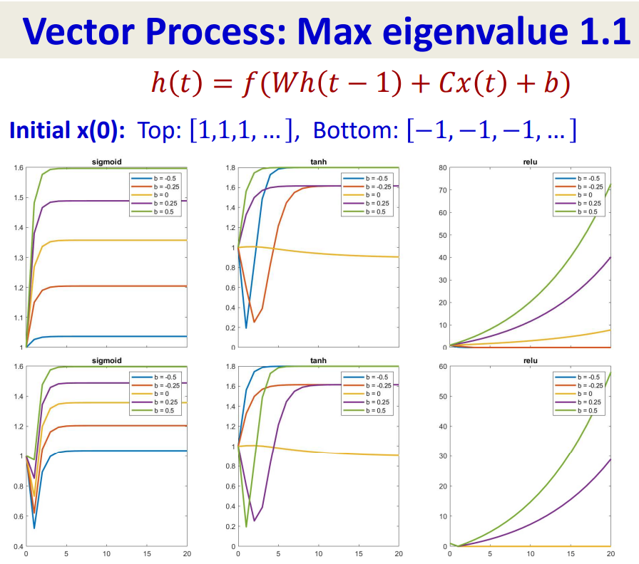
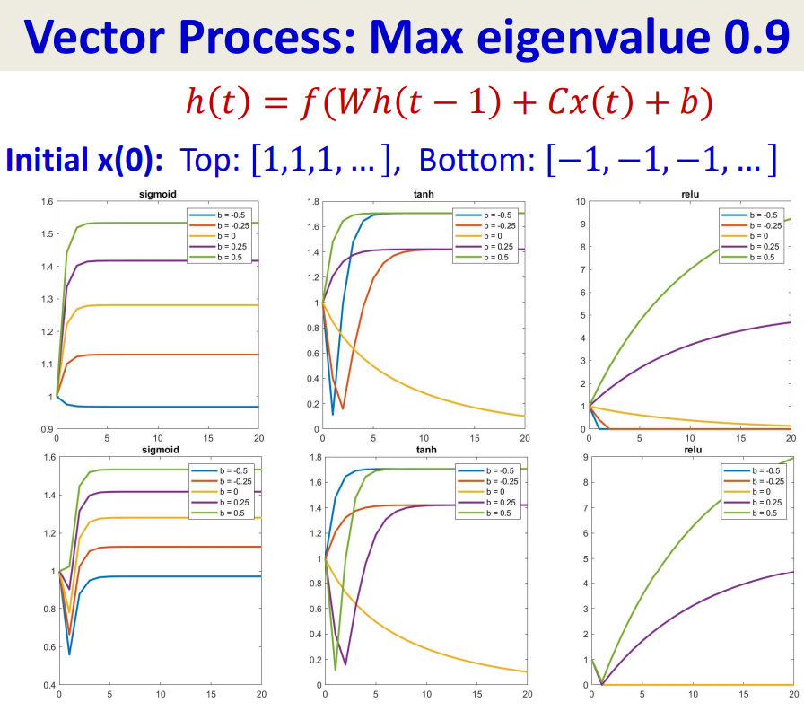
So Tanh activations are slightly more effective at storing memory, but they too not for very long (the inputs are eventually forgotten in an exponential manner).

Exploding & Vanishing Gradients

We know about the vanishing gradients problem in MLPs — that for most common activation functions which have derivatives always less than 1, multiplication by the Jacobian is always a shrinking operation. Because of this, the derivative of divergence after a few layers at any time is totally forgotten.

Effect of weights:

Each weight matrix $W_n$ performs a linear transformation of the gradient. Specifically:

It scales the gradient in different directions.
The amount of scaling is determined by the singular values (or eigenvalues for symmetric matrices) of the matrix.

Let’s say the singular values of a matrix $W_n$ are $\sigma_1, \sigma_2, \ldots, \sigma_m$

If all $\sigma_i<1 \rightarrow$ gradient will shrink in all directions
If any $\sigma_i > 1 \rightarrow$ gradient may grow in that direction

If many weight matrices have singular values greater than 1, then the gradients will explode.

If many weight matrices have singular values lesser than 1, then the gradients will vanish.

Important points:

The derivatives for most parameters will become vanishingly small as we backpropagate the loss gradient through deep networks
The derivatives for a small number of parameters will blow up and become large and unstable as we propagate the los gradient through deep networks
The derivatives would be more stable if the recurrent weight matrices had singular values equal to 1
The derivatives would be more stable if the recurrent activations were identity transforms (with identity Jacobian matrices)
The memory would be more stable if the recurrent weight matrix were an identity matrix (i.e. a diagonal matrix with diagonal values equal to “1”)
The memory would be more stable if the recurrent activations were identity transforms (which are linear and do not scale up or shrink the output)

LSTM

We want the RNN to remember for extended periods of time and recall when necessary by tackling the expanding and vanishing gradients problem.

We do this by getting rid of the Jacobian and weight matrices, but we retain memories until a switch based on the input flags them as okay to forget, and recall them on demand.

This is called the constant error carousel — they have something in memory, and at each time $t$, what is in memory is modified based on what is encountered in the input.

The Long Short-Term Memory neuron allows us to explicitly latch information to prevent decay and blowing up of gradients.

GRU

Time-Synchronous Recurrence

They have one output corresponding to every input. They can be bidirectional as well.

Assumption: Sequence divergence is the sum of the divergence at individual instants

\[Div(Y_{target}(1 ... T), Y(1 ... T)) = \Sigma_t Div(Y_{target}(t), Y(t))\] \[∇_{Y(t)} Div(Y_{target}(1 ... T), Y(1 ... T)) = ∇_{Y(t)} Div(Y_{target}(t), Y(t))\]

Typical divergence for classification:

\[Div(Y_{target}(t), Y(t)) = KL(Y_{target}(t), Y(t))\]

Variants

These are all sequence to sequence models, and we will soon transition into a separate heading to tackle these problems, specifically on training them.

Many to One:

Consider a many to one RNN. In such networks:

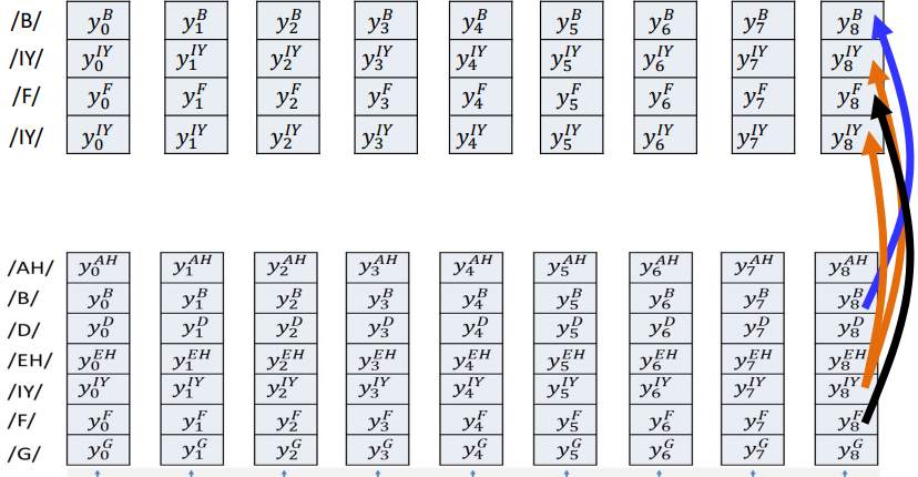
Even though we only read the final output at the end of the sequence, every hidden state at each time step does generate an output internally.
These outputs are typically ignored during inference, unless you’re doing something like attention or intermediate supervision.

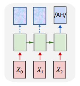
During training, the divergence (loss) is only computed at the final step.

We define the divergence as the KL divergence between the target phoneme and the predicted output at the final time step:

\[DIV(Y_{\text{target}}, Y) = KL(Y(T), \text{Phoneme})\]

This approach assumes that the only useful information is at the final step. But intermediate states may have rich information too! So we’re wasting learning potential by ignoring outputs from intermediate inputs.

So the solution to this is to use all outputs generated during the forward pass — not just the final one — to compute divergence. That is, assume that each hidden state output should try to predict the same target phoneme. So instead of just computing divergence at $t=T$, we compute it for all $t \in {0,1,2}:$

\[DIV(Y_{\text{target}}, Y) = \sum_t w_t \cdot KL(Y(t), \text{Phoneme})\]

$w_t$ is a weighting factor for each time step. You can keep them equal, or weigh later steps more if needed.

Many to One:

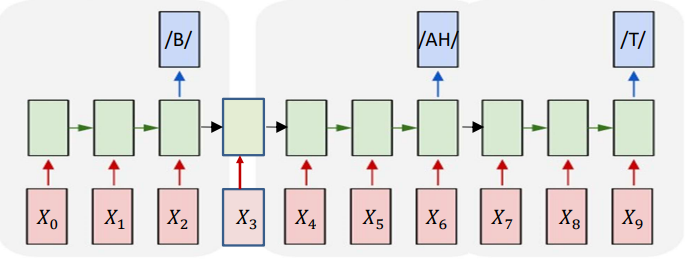
Objective: Given a sequence of inputs, asynchronously output a sequence of symbols.

This is just a simple concatenation of many copies of the simple “output at the end of the input sequence” model discussed above.

But during inference, the network is producing an output at every time and we need to figure out when to read the outputs because we are not given this information. This process of obtaining an output from the network is called decoding.

Solution to decoding:

Option 1:

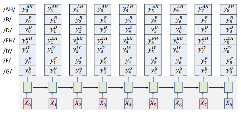
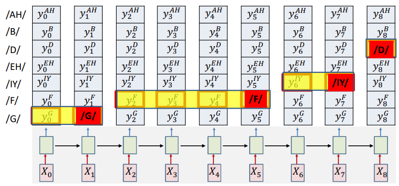
At each time, the network outputs a probability for each output class given all inputs until that time.

\[y_k^D = prob(s_4=D|X_0\ldots X_k)\]

Just like we do in any neural network with a softmax or logistic output, we select the class with the highest probability results. Using the same principle here, we find the most likely symbol sequence at each time given the inputs. Then we merge adjacent repeated symbols, and place the actual emission of the symbol in the final instant.

# Pseudo-code
# Assuming y(t,i), t = 1...T, i = 1...N is already computed using the underlying RNN
# N is the number of classes in output

n = 1
best(1) = argmax_i y(1, i)
for t = 1 to T:
    best(t) = argmax_i y(t, i)
    if best(t) != best(t-1):
        out(n) = best(t-1)  # stores the previous class (the segment that just ended)
        time(n) = t - 1     # stores the time it ended
        n = n + 1

But the problem with this is that we cannot distuinguish between an extended symbol and repetitions of symbols.

Sequence-to-Sequence Models

Training

During training, if we have the input sequences and also the output sequence, i.e., at what exact time step we have a label, then training becomes easy. We can then easily convert it into a time-synchronous problem and train the model.

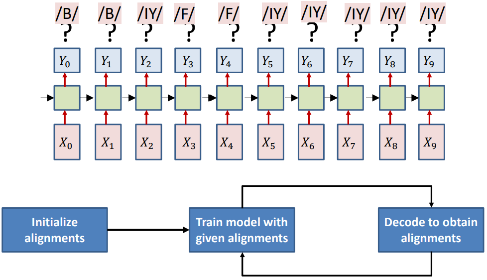
But the problem arises when no timing information of the output is provided. Only the sequence of output symbols is provided for the training data, but there is no indication of which one occurs where. This becomes a problem of “training without alignment”, and can be solved in two ways:

Guess the alignment — Viterbi algorithm
Consider all possible alignments — Connectionist Temporal Classification

Formally, we want to solve:

Given an unaligned $K$ length compressed symbol sequence $S = s_0, \dots, s_{K-1}$, and an $N$ length input $(N\geq K)$, we want to find the most likely alignment:

\[\argmax_{s_0, \dots, s_{N-1}} \Pr(s_0, \dots, s_{N-1} \mid S, X)\quad \text{such that} \quad \text{compress}(s_0, \dots, s_{N-1}) = S\]

The expression inside the $\text{argmax}$ represents the model’s belief about the alignment. The constraint ensures that the sequence, once compressed, matches the given label sequence.

Important points:

Alignment tells us which portion of the input aligns with what symbol in the sequence
An order-synchronous symbol sequence that is shorter than the input can be “aligned” to the input by repeating symbols until the expanded sequence is exactly as long as the input
The “alignment” of an order-synchronous symbol sequence to an input is a time synchronous symbol sequence
A symbol sequence that is time-synchronous with an input can be compressed to a shorter order-synchronous input by eliminating repetitions of symbols
Order-synchronous symbol sequences that are shorter than the input are compressed symbol sequences

Training: Guessing the Alignment using Viterbi Algorithm

When the alignment is not provided, one approach is to guess it and refine it iteratively. Procedure:

Initialize: Assign an initial alignment (can be random, heuristic-based, uniform, etc.)
Train: Train the network using the current alignment
Re-estimate: Update the alignment based on the model’s improved predictions
Repeat steps 2-3 until convergence

When a model outputs a distribution over symbols at each time step, greedy decoding (i.e., taking the highest probability symbol at each step) can produce invalid outputs.

To tackle this, we prune the model’s output grid and retain only the rows corresponding to symbols that occur in the target sequence. This gives us a reduced output table, eliminating unwanted paths. This assures that we only hypothesize symbols that are valid, but it still doesn’t enforce their correct order.

To ensure that the output expands the target sequence exactly, we:

Create one row per symbol in the output sequence — If a symbol repeats, create multiple rows
Arrange the rows in the desired order
Build a table such that at each time step, you have probabilities for that symbol

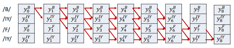
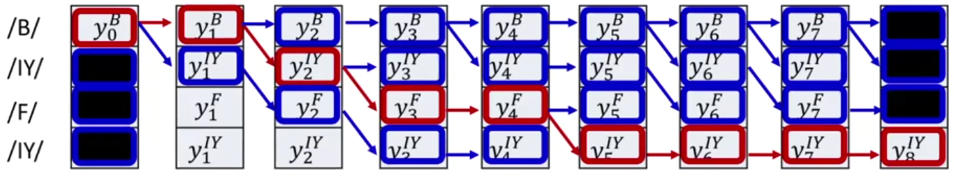
This ensures the alignment can only traverse through the correct symbol order. Once the output table is arranged, we model it as a graph:

Rows represent the positions of target symbols
Columns represent time steps $t=0,1,\ldots,T-1$
Nodes contain the network’s output scores for the corresponding symbol at time $t$:
\[y_t^{s_i} = \text{Pr}(s_i|x_0,\ldots,x_t)\]
Edges have a score of $1$ and connect a node to:
- The next time step on the same row (symbol is held)
- The next row (next symbol) at the next time step

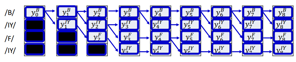
We define valid paths to:

Start at top-left
End at bottom-right
Monotonically move downward or forward in time

Graph constraints:

To ensure valid decoding, we impose these:

The first symbol must begin at the top-left node.
The last symbol must end at the bottom-right node.
All paths must be monotonic:
- You can stay on the same row (repeat symbol)
- Or move downward to the next symbol (progress in output)
- But you can’t go backward

This guarantees that the path represents a valid expansion of the target sequence.

Scoring Paths:

Each path through the graph represents a possible alignment. The score of a path is the product of the probabilities of its nodes:

\[\text{Score(Path)} = \prod_{(t, i) \in \text{Path}} y_t^{s_i}\]

This score represents the model’s confidence in that specific alignment.

To pick the most likely alignment given the input and given this graph, we need to pick the path that has the highest probability.

Using this, we can find the most probable path from source to sink using any dynamic programming algorithm, such as breadth-first search, Dijkstra’s, A*, etc. One such algorithm is the Viterbi algorithm.

Viterbi Algorithm

The basic idea is that the best path to any node must be an extension of the best path to one of its parent nodes. Any other path would necessarily have a lower probability.

The best parent is simply the parent with the best scoring best path.

Algorithm:

Dynamically track the best path (and the score of the best path) from the source node to every node in the graph
- At each node, keep track of:
  - The best incoming parent edge
  - The score of the best path from the source to the node through this best parent edge
Eventually compute the best path from source to sink

Pseudocode:

Initialization
\[BP(0, i) = \text{null}, \quad i = 0, \ldots, K-1\] \[Bscr(0,0) = y_0^{S(0)}, \quad Bscr(0,i) = -\infty, \quad i = 1, \ldots, K-1\]
For $t = 1, \ldots, T-1$
\[BP(t,0) = 0, \quad Bscr(t,0) = Bscr(t-1,0) \times y_t^{S(0)}\]
- For $l = 1, \ldots, K-1$
  \[BP(t,l) = \begin{cases} l-1, & \text{if } Bscr(t-1,l-1) > Bscr(t-1,l) \\ l, & \text{otherwise} \end{cases}\] \[Bscr(t,l) = Bscr(BP(t,l)) \times y_t^{S(l)}\]

$s(T-1) = s(K-1)$
for $t=T-1:1$
- $s(t-1) = BP(s(t))$

Loss:

\[DIV = \sum_t KL(Y_t, symbol_t^{bestpath}) = -\sum_t \log Y(t, symbol_t^{bestpath})\] \[\nabla_{Y_t} DIV = \begin{bmatrix} 0 & 0 & \cdots & \frac{-1}{Y(t, symbol_t^{bestpath})} & 0 & \cdots & 0 \end{bmatrix}\]

The gradient is zero everywhere except at the component corresponding to the target in the estimated alignment. This shows that only the probabilities along the best path (red boxes) receive gradient updates.

Problem with Iterative Update:

Approach is heavily dependent on initial alignment
Prone to poor local optima
The process works well if we have large amounts of training data

Alternate solution: Do not commit to an alignment during any pass

Training: Connectionist Temporal Classification

Instead of only selecting the most likely alignment, we use the statistical expectation over all possible alignments.

\[DIV = \mathbb{E} \left[ -\sum_t \log Y(t, s_t) \right]\]

We want to train a model that outputs, at each frame $t$, a probability distribution $Y_t(.)$ over symbols.

We are given an unaligned label sequence $\mathbf{S} = S_0, S_1, …, S_{K-1}$ and an input frame sequence $\mathbf{X} = X_0, X_1, …, X_{N-1}$.

Because alignment is unknown, there are many ways to align $\mathbf{S}$ to the frames. Instead of picking one alignment (best path), we average over all valid alignments. Concretely, we need the probability that a particular symbol $s$ is aligned to frame $t$, given $\mathbf{S,X}$. That probability is:

\[P(s_t=S|\mathbf{S},\mathbf{X})\]

Another way of explaining this is that this is the posterior (conditional) probability that the model is aligned with symbol $S$ at time $t$, given that we already know the model should produce the overall label sequence $\mathbf{S}$, and we have the input $\mathbf{X}$. Or, given that the model correctly produces the target sequence $\mathbf{S}$, what’s the chance that, at frame $t$, it’s currently aligned to symbol $S$.

From expectation to a computable loss:

Start from the expectation over alignments:

\[DIV = \mathbb{E} \left[ -\sum_t \log Y(t, s_t) \right]\]

This expectation can be written using the frame-label posterior $P(s_t=S|\mathbf{S},\mathbf{X})$:

\[DIV = -\sum_{t}\sum_{s\in{S_0,\dots,S_{K-1}}} P(s_t=S\mid \mathbf{S},\mathbf{X})\log Y(t,s_t={S})\]

So training reduces to two things:

compute the posteriors $P(s_t=S|\mathbf{S},\mathbf{X})$ for every $t,s$
take a weighted cross-entropy using those posteriors as targets

How do we compute $P(s_t=S|\mathbf{S},\mathbf{X})$?

\[P(s_t=S|\mathbf{S_r},\mathbf{X}) \propto P(s_t=S_r, \mathbf{S}|\mathbf{X})\]

$P(s_t=S_r, \mathbf{S}|\mathbf{X})$ is the joint probability that:

At time $t$, the model is aligned with symbol $S_r$
and over the entire sequence, the model emits (or aligns to) the full target label sequence $\mathbf{S}$

Intuitively, this answers what is the total probability that, while generating the entire target sequence $\mathbf{S}$, the model goes through symbol $S_r$ at time $t$.

To compute this efficiently, we split the trellis into two parts:

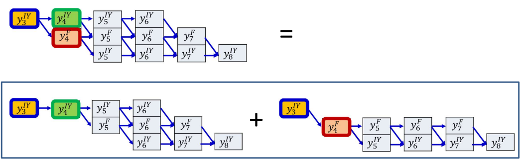
\[P(s_t = S_r, S \mid X) = P(S_0, ..., S_r, s_t = S_r \mid X) \times P(S_{t+1}, ..., S_{K-1} \mid S_0, ..., S_r, s_t = S_r, X)\]

The first path

\[P(S_0, ..., S_r, s_t = S_r \mid X)\]

represents the probability of all partial paths that lead up to state $S_r$ at time $t$. This is the forward probability, denoted by $\alpha_t$.

\[\alpha(t, r) = P(S_0, S_1, ..., S_r, s_t = S_r \mid X)\]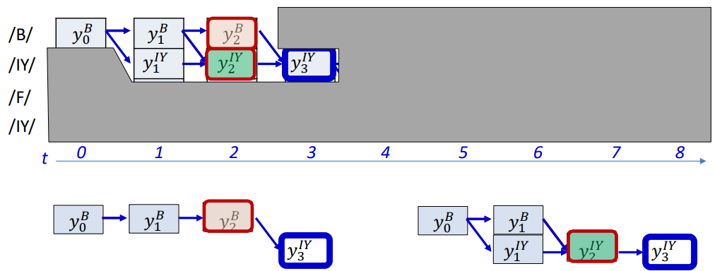

This is the total probability of all valid paths that align the prefix of the target sequence up to symbol $S_r$ to the first $t$ input frames, and that end exactly at symbol $S_r$ at time $t$.

\[\alpha(t, r) = \sum_{q : S_q \in pred(S_r)} \alpha(t-1, q) Y_t^{S(r)}\]

$pred(S_r)$ is the set of symbols that are allowed to transition into $S_r$. It usually includes itself (stay transition) and the previous symbol (advance transition)
$q$ is its row index
$Y_t^{S(r)}$ is the network’s predicted probability of symbol $S_r$ at time $t$
$\alpha(t-1,q)$ is the total probability of reaching predecessor $S_q$ at the previous frame

The second part

\[P(S_{t+1}, ..., S_{K-1} \mid S_0, ..., S_r, s_t = S_r, X)\]

represents the probability of all possible continuations after time $t$ that follow valid transitions and end in the final symbol. This is the backward probability, denoted by $\beta_t$.

\[\beta(t, r) = P(\text{rest of the path from } (t, r) \text{ to the end} \mid X)\]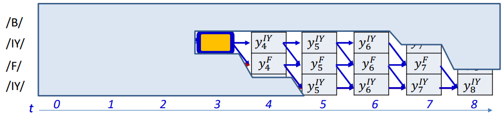

$\beta(t,r)$ is the total probability of all valid paths that start after time $t$, given that you are currently at state $S_r$ at time $t$, and that follow legal transitions until the sequence ends.

$\beta(t,r)$ is the probability of the exposed subgraph, not including the orange shaded box. For convenience, let us include the box in the graph, and factor it out later.

$\hat{\beta}(t,r)$ is the probability of graph including node at $(t,r)$.

\[\beta(t, r) = \frac{1}{y_t^{S_r}} \hat{\beta}(t, r)\] \[\hat{\beta}(t, r) = y_t^{S_r} \sum_{q \in succ(r)} \hat{\beta}(t+1, q)\]

$succ(r)$ is the set of successor states that can follow $S_r$
$y_t^{S_r}$ emission probability of symbol $S_r$ at time $t$

\[\beta(t, r) = \frac{\hat{\beta}(t, r)}{y_t^{S_r}}\]

To get the posterior probability (the fraction of total path probability passing through this node):

\[P(s_t = S_r \mid S, X) = \frac{\alpha(t,r)\beta(t,r)}{\sum_j \alpha(t,j)\beta(t,j)}\]

Finally, putting all this back into the expected divergence

\[DIV = -\sum_{t}\sum_{s\in{S_0,\dots,S_{K-1}}} P(s_t=S\mid \mathbf{S},\mathbf{X})\log Y(t,s_t={S})\]

Forward Algorithm

Initialization
\[\alpha(0,0) = y_0^{S(0)}, \quad \alpha(0,r) = 0, r > 0\]
$\text{for } t = 1, \ldots, T-1$:
\[\alpha(t,0) = \alpha(t-1,0) y_t^{S(0)}\]
- $\text{for } l = 1, \ldots, K-1$:
  \[\alpha(t,l) = \big(\alpha(t-1,l) + \alpha(t-1,l-1)\big) y_t^{S(l)}\]

Backward Algorithm

Initialization
\[\hat{\beta}(T-1, K-1) = y_{T-1}^{S(K-1)}, \quad \hat{\beta}(T-1, r) = 0, r < K-1\]
$\text{for } t = T-2 \text{ downto } 0$
- $\text{for } r = K-1 \text{ downto } 0$
  \[\hat{\beta}(t, r) = y_t^{S(r)} \sum_{q \in succ(r)} \hat{\beta}(t+1, q)\] \[\beta(t, r) = \frac{1}{y_t^{S(r)}} \hat{\beta}(t, r)\]

Tackling Repetitions

Inference

Language Models

Language Models (LMs) model the probability distribution of token sequences in a language. For example, word sequences, if words are the tokens.

LMs can be used to:

Compute the probability of a given token sequence
Generate new sequences from the learned distribution of the language

A language model assigns a probability to an entire sequence of tokens (words, subwords, characters). If your sentence is $(w_1,w_2,w_3,…)$, the LM’s job is to say how likely that whole sequence is. Because directly modeling $P(w_1,w_2,…,w_T)$ is hard, we use the chain rule of probability to factor it into conditional next-token probabilities:

\[P(w_1, w_2, \ldots, w_T) = \prod_{t=1}^{T} P\left(w_t \mid w_1,\ldots,w_{t-1}\right)\]

Representing Words

Words are represented as one-hot vectors. We pre-specify a vocabulary $V$ of $N$ words in a fixed (e.g., lexical) order. Example: V = [ A, AARDVARK, AARON, ABACK, ABACUS, …, ZZYP ]

Each word $w \in V$ is mapped to a vector $\mathbf{e}_w \in \mathbf{R}^N$ with all zeros except a single 1 at that word’s index. If “ARRON” is index 3,

\[\mathbf{e}_{ARRON} = [0, 0, 1, 0, ..., 0]\]

Characters can be encoded the same way with a smaller $N (\approx 100$ for English if you include case, punctuation, digits, symbols, and space).

Why use one-hot representation?

It makes no assumptions about the relative importance of words. All word vectors are the same length
It makes no assumptions about the relationships between words
The distance between every pair of words is the same

Why one-hot is not enough?

Sparsity & dimensionality
- Vectors are length $N$ and almost entirely zero.
- Memory & compute scale with $N$. With a 100k-word vocab, each vector is 100k-dimensional.
- It uses only $N$ corners of the $2^N$ corners of a unit cube.
No notion of similarity
- Any two distinct one-hots have cosine similarity $0$ and Euclidean distance $\sqrt{2}$. “cat” and “dog” are as dissimilar as “cat” and “banana.”
- So the model must learn from scratch that some words are related.
UNK problem
- It is not possible to include every possible word in your vocabulary $V$.
- You fix $V$(say, 50 000 most frequent tokens). Anything not in $V$, such as a new name, misspelling, slang, or foreign word, is replaced by a special [UNK] token (“unknown”).

Solution to the dimensonality problem: Embeddings

The goal is to reduce the dimensonality of one-hot vectors while preserving semantic relationships among words.

Each work $W$ (a one-hot vector) is projected into a smaller, dense vector using a learned projection matrix $P$:

\[W \rightarrow P W\]

Here,

$W$ is the one-hot vector of dimension $N$
$P$ is the projection matrix of size $M \times N$, where $M « N$
$PW$ is the new dense vector representation (embedding) of dimension $M$

Intuition:

This is a linear transformation into a lower-dimensional space
Each original axis (word) is now represented as a point in this smaller subspace
If trained properly, distances between projected points will correspond to semantic similarity between words

Benefits of projection:

Reduces computational complexity drastically
Converts sparse high-dimensional one-hots into dense, meaningful embeddings
Word similarity (e.g., “cat” and “dog”) becomes measurable via cosine similarity or Euclidean distance

Embeddings, however, still don’t enable you to find representations for words that are not part of our training vocabulary.

Each word’s one-hot vector $W_i$ is multiplied by $P$ to get its embedding:

\[PW_i = \text{embedding of word } W_i\]

Then, a function $f(.)$ predicts the next word based on the embeddings of the previous words:

\[W_n = f(PW_0, PW_1, ..., PW_{n-1})\]

$P$ is shared across all words — it’s a single learned matrix
The same transformation is applied to every word’s one-hot vector
$f$ can be a neural network that learns to combine embeddings from context words
$P$ is updated during training, so embeddings gradually become semantically meaningful

Mathematically, $P$ acts as a linear layer with $M$ outputs and $N$ inputs:

\[\text{Embedding} = P W = E[w]\]

This can be implemented as:

A linear transformation shared across all inputs, or
A lookup operation in an embedding table (each row is one projected vector).

Beginnning and End of Sentences

A sequence of words by itself does not indicate if it is a complete sentence or not. To make it explicit, we will add two additional symbols (in addition to the words) to the base vocabulary.

<sos> Indicates start of a sentence
<eos> Indicates end of a sentence

In situations where the start of sequence is obvious, the <sos> may not be needed, but <eos> is required to terminate sequences.

So when predicting the next token, we feed the drawn word as the next word in the series by sampling from the output probability distribution. We continue this process until we draw an <eos>, or if we decide to terminate generation based on some other criterion.

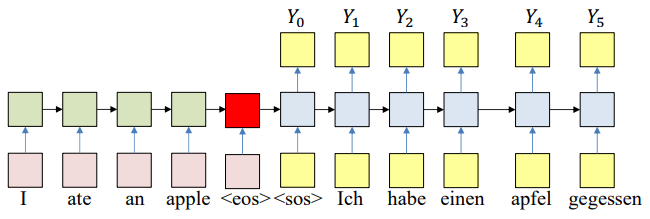
Delayed Sequence to Sequence Models

Pseudocode:

# --- Step 1: Encode the input sequence ---
# First run the inputs through the network  
# Assuming h(-1,1) is available for all layers  

for t = 0 : T-1                      # Including both ends of the index  
    [h(t), ...] = RNN_input_step(x(t), h(t-1), ...)  
H = h(T-1)                            # Final hidden state after reading all inputs  

# --- Step 2: Generate the output sequence ---
# Now generate the output y_out(1), y_out(2), ...  

t = 0  
h_out(0) = H  

do  
    t = t + 1  
    [y(t), h_out(t)] = RNN_output_step(h_out(t-1))  
    Y_out(t) = draw_word_from(y(t))  
until Y_out(t) == <eos>  

# --- Explanation ---
# x(t)        : input at time step t (e.g., word embedding)
# h(t)        : hidden state carrying memory of previous inputs
# H           : final hidden state summarizing the input sequence
# RNN_input_step()  : recurrence for encoding
# RNN_output_step() : recurrence for decoding
# draw_word_from()  : selects the most likely or sampled word
# <eos>       : end-of-sequence token signaling generation stop

Encoder network:
- The input sequence feeds into a recurrent structure
- The input sequence is terminated by an explicit <eos> symbol
- The hidden activation at the <eos> “stores” all information about the sentence
Decoder network:
- Subsequently a second RNN uses the hidden activation as initial state, and <sos> as initial symbol, to produce a sequence of outputs
- The output at each time becomes the input at the next time
- Output production continues until an <eos> is produced

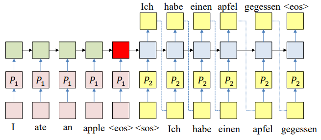
The one-hot word representations can also be compressed via embeddings. These embeddings will be learned along with the rest of the network.

At each time $k$ the network produces a probability distribution over the output vocabulary

\[y_k^w = P(O_k=w | O_{k-1}, ..., O_1, I_1, ..., I_N)\]

At each time a word is drawn from the output distribution and is provided as an input to the next time. Over the entire predicted sequence, we compute the total probability as

\[P(O_1, ..., O_L \mid I_1, ..., I_N) = P(O_1 \mid I_{1}, ..., I_N) P(O_2 \mid O_1, I_1, ..., I_N) P(O_3 \mid O_1, O_2, I_1, ..., I_N) ... P(O_L \mid O_1, ..., O_{L-1}, I_1, ..., I_N) = y_1^{O_1} , y_2^{O_2} , ... , y_L^{O_L}\]

Picking the next token given the probability distribution

The model gives a distribution $y_t$ at each time step $t$. The ideal decoder would pick the sequence

\[\arg\max_{o_{1:L}} \prod_{t=1}^{L} y_t^{(o_t)}\]

i.e., the most probable sequence as a whole, not just the best token at each step. That’s hard to search exactly, so we approximate.

Greedy decoding:

At each step, choose the token with the highest probability in $y_t$, feed it back, and repeat until <eos>.

Why this often fails?

Myopia: A locally best token can push the model into a worse future. Example: choosing “he” at $t=0$ might make “nose” at $t=1$ more likely than a better global path (“knows” later).
Distribution shaping: The token you pick changes the next distribution. Sometimes picking a slightly less likely token now makes the next distribution much “peakier,” yielding a higher overall product of probabilities.
Error compounding: One early poor choice can lock you into a suboptimal continuation.

Sampling:

At each step, sample a token from the full distribution $y_t$. It introduces diversity and can escape greedy’s local traps. It also sometimes stochastically finds better (higher-probability) sequences than greedy.

Why it also fails?

Unreliable: You may sample low-probability “junk” early, which can derail future steps
High variance: Two runs can differ wildly; average quality can drop without constraints.

What is actually used in practice?

Beam search: Keep the top-$B$ partial sequences at each step (by cumulative log-probability), expand each, prune again.
Top-k sampling: At each step, restrict to the $k$ most probable tokens (renormalize), then sample.
Nucleus (Top-p) Sampling: Choose the smallest set of tokens whose cumulative probability $\ge p$, renormalize, sample.

Beam Search

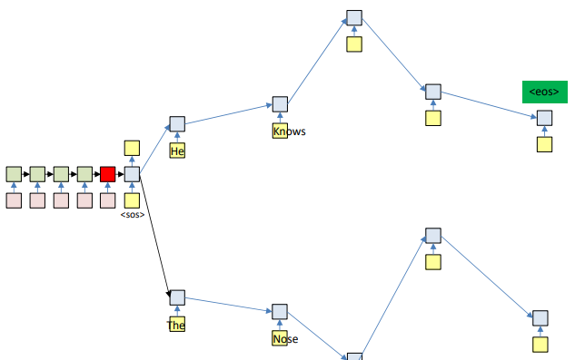
At each time step, the model can produce many possible next words. If we try to explore all of them, the search tree explodes exponentially (like “He knows…” vs. “The nose…”). So, the idea is to prune — keep only the top few promising paths instead of exploring everything.

We compute the cumulative probability for each partial sequence up to time $t$:

\[P(O_1, ..., O_t \mid I_1, ..., I_N) = \prod_{n=1}^{t} P(O_n \mid O_{1:n-1}, I_1, ..., I_N)\]

At every time step, we:

Expand each of the current candidate sequences by all possible next words.
Compute their cumulative probabilities (product of conditional probabilities).
Retain only the top K candidates (where K is called the beam width).

The search continues until one of the active hypotheses produces an <eos> token. We can employ one of two strategies:

Early termination: Stop as soon as the most likely overall path ends with <eos>. This is used for fast inference.
N-best search: Continue expanding other beams even after some reach <eos> to collect multiple high-probability completions. This is used in translation or summarization tasks.

Once a path emits the <eos> token, it cannot be extended further — it’s a completed sequence. Different beams may terminate at different lengths. The final output is the sequence ending with <eos> that has the highest cumulative probability across all terminated beams.

Pseudocode:

# Assuming encoder output H is available
path = <sos>
beam = {path}
pathscore = [path] = 1
state[path] = h[0]   # Output of encoder

do  # Step forward
    nextbeam = {}
    nextpathscore = {}
    nextstate = {}

    for path in beam:
        cfin = path[end]
        hpath = state[path]
        [y, h] = RNN_output_step(hpath, cfin)

        for c in Symbolset:
            newpath = path + c
            nextstate[newpath] = h
            nextpathscore[newpath] = pathscore[path] * y[c]
            nextbeam += newpath   # Set addition
        end
		end
    beam, pathscore, state, bestpath = prune(nextstate, nextpathscore, nextbeam, bw)
until bestpath[end] == <eos>

function prune(state, score, beam, beamwidth):
    sortedscore = sort(score)
    threshold = sortedscore[beamwidth]

    prunedstate = {}
    prunedscore = {}
    prunedbeam = {}

    bestscore = -inf
    bestpath = None

    for path in beam:
        if score[path] > threshold:
            prunedbeam += path     # Set addition
            prunedstate[path] = state[path]
            prunedscore[path] = score[path]

            if score[path] > bestscore:
                bestscore = score[path]
                bestpath = path
            end
        end
    end
    return prunedbeam, prunedscore, prunedstate, bestpath

Training

Forward Pass

Input the source and target sequences, sequentially. The output will be a probability distributon over target symbol set (vocabulary).

Backward Pass

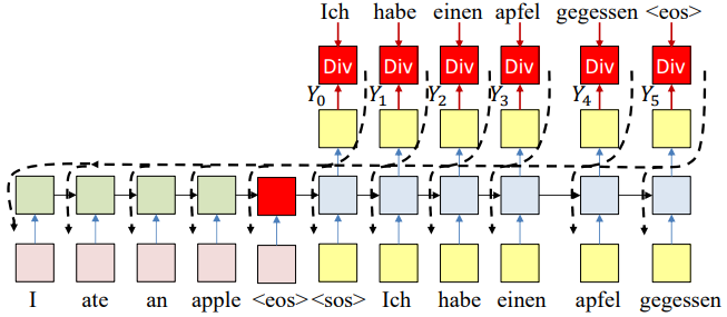
We compute the divergence between the output distribution and target word sequence. Then we backpropagate the derivatives of the divergence through the network to learn.

In practice, if we apply SGD, we may randomly sample words from the output to actually use for the backprop and update.

Deep Learning - CNNs, RNNs, & Language Models

To-Do

Convolutional Neural Networks

Forward Pass

Backpropagation

Recurrent Neural Networks

State-Space Model

Variants on RNNs

Training

Forward Pass

Back Propagation Through Time (BPTT)

Bidirectional RNN

Inference

Forward Pass

Back Propagation Through Time

Behavior of Recurrence

BIBO Stability

Exploding & Vanishing Gradients

LSTM

GRU

Time-Synchronous Recurrence

Variants

Sequence-to-Sequence Models

Training

Important points:

Training: Guessing the Alignment using Viterbi Algorithm

Viterbi Algorithm

Training: Connectionist Temporal Classification

Forward Algorithm

Backward Algorithm

Tackling Repetitions

Inference

Language Models

Representing Words

Solution to the dimensonality problem: Embeddings

Beginnning and End of Sentences

Delayed Sequence to Sequence Models

Picking the next token given the probability distribution

Beam Search

Training

Forward Pass

Backward Pass

Further Reading

Deep Learning - Attention & Transformers

Deep Learning - Perceptrons

Deep Learning