Diffusion and Flow Matching

Diffusion and Flow Matching Notes

This blog is a collection of my notes based on the MIT lecture series: Introduction to Flow Matching and Diffusion Models.

Flow and Diffusion Models

Flow Models

Ordinary Differential Equations

An ordinary differential equation (ODE) describes how a point moves through space over time. A solution to an ODE is defined by a trajectory, which is a function

\[{X}:[0,1] \rightarrow \mathbb{R}^d, \quad t \mapsto X_t\]

that maps from time $t \in [0,1]$ to some location in space $X_t \in \mathbb{R}^d$. Here, $X_t$ is a random variable whose value is the particle’s location $x$ at time $t$, and $x$ is a location in space (a coordinate where we evaluate densities and vector fields).

Every ODE is defined by a vector field $u$, which is a function of the form

\[u : \mathbb{R}^d \times [0,1] \to \mathbb{R}^d, \quad (x,t) \mapsto u_t(x)\]

i.e. for every time $t$ and location $x$ we get a vector $u_t(x) \in \mathbb{R}^d$ specifying a velocity in space. In other words, $u_t(x)$ is the velocity that any particle would have if it were located at position $x$ at time $t$.

An ODE imposes a condition on a trajectory: we want a trajectory $X$ that “follows along the lines” of the vector field $u_t$, starting a the point $x_0$,

\[\frac{d}{dt} X_t = u_t(X_t)\] \[X_0 = x_0\]

The first equation requires that the derivative of $X_t$ is specified by the direction given by $u_t$. The second part of it requires that we start at $x_0$ at time $t=0$.

Intuition: This of this river analogy:

• The vector field $u$ is the map of the water’s velocity: at every point in the river, an arrow shows the direction and speed.
• The trajectory $X$ is the path of a leaf dropped at $x_0$, carried along by the current. The leaf has no choice but to follow wherever the water pushes it.

The Flow

Given the trajectory interpretation, a natural question arises: if we start at $X_0 = x_0$, where do we end up at time $t$? This question is answered by the flow, a function

\[\psi : \mathbb{R}^d \times [0,1] \to \mathbb{R}^d, \quad (x_0,t) \mapsto \psi_t(x_0)\]

satisfying

\[\frac{d}{dt}\,\psi_t(x_0) = u_t(\psi_t(x_0))\] \[\psi_0(x_0) = x_0\]

$\psi_t(x_0)$ is the position at time $t$ of a particle that started at $x_0$. The trajectory for a given initial condition is recovered as

\[X_t = \psi_t(X_t)\]

Intuition: The river analogy extends: the vector field $u$ is the velocity map, the trajectory $X$ is the path of one specific leaf, and the flow $\psi$ is the “big picture” function: it describes where any leaf starting anywhere will end up after any amount of time. It is a map of space itself.

So vector fields, ODEs, and flows are three descriptions of the same object. Vector fields define ODEs; ODEs have solutions that are flows.

A Concrete Example: Linear Vector Fields

To make the ODE machinery concrete, consider the simple linear vector field

\[u_t(x) = -\theta x, \quad \theta>0\]

This is a vector field that always points toward the origin, with strength proportional to distance from the origin. The flow solving this ODE is

\[\psi_t(x_0) = e^{-\theta t} x_0\]

We can verify this satisfies both conditions:

• First, at $t=0$, $\psi_0(x_0)=e^0x_0=x_0$, which satisfies the initial condition.

• Second,

  \[\frac{d}{dt}\,\psi_t(x_0) = \frac{d}{dt}\left(e^{-\theta t} x_0\right) = -\theta e^{-\theta t} x_0 = -\theta \psi_t(x_0) = u_t(\psi_t(x_0))\]

  which satisfies the ODE.

The flow converges exponentially to the origin as $t \rightarrow \inf$, collapsing all starting points toward zero.

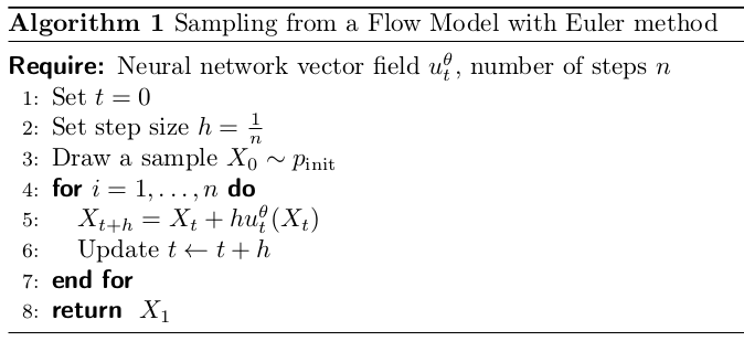
Simulating an ODE: The Euler Method

The Flow Model

We now have everything needed to define a generative model using an ODE. The idea is elegant: we use the ODE to transform noise samples from $p_{\text{init}}$ into data samples from $p_{\text{data}}$ by choosing the vector field $u$ appropriately.

A flow model is defined by:

\[X_0 \sim p_{\text{init}}\] \[\frac{d}{dt} X_t = u_t^\theta(X_t)\]

where $u_t^\theta$ is a neural network with parameters $\theta$. The network takes as input a position $x\in \mathbb{R}^d$ and a time $t \in [0,1]$, and outputs a velocity vector in $\mathbb{R}^d$. The training objective is to choose $\theta$ so that the endpoint $X_1$ of the trajectory has a distribution $p_{\text{data}}$:

\[X_1 \sim p_{\text{data}} \;\Longleftrightarrow\; \psi_1^\theta(X_0) \sim p_{\text{data}}\]

where $\psi_t^\theta$ is the flow induced by $u_t^\theta$.

Note: The neural network parameterizes the vector field, not the flow. To compute the flow, we must simulate the ODE. The network only defines how points move locally at each moment; the global transformation emerges from integrating that local motion over time.

A flow model samples noise once at $t=0$, then deterministically moves each point using the learned velocity field. The entire trajectory is deterministic given the initial noise sample. The collection of endpoints, one per noise sample, should match the data distribution.

Intuition: Consider an image generation case.

• $X_0$ is the entire noise image (all pixels sampled from Gaussian) and is one vector in $\mathbb{R}^{H \times W \times 3}$.
• $X_1$ is the final generated image. Same space, but now looks like a real photo.
• $p_{\text{data}}$ the implicit distribution over all natural images, defined by your training dataset. A dog photo has high probability; pure noise has near zero.
• The flow: the continuous sequence of intermediate images $X_0 \to X_{0.1} \to \cdots \to X_1$. Each $X_t$ is a full image that looks like a partially-denoised blur, gradually becoming coherent.
• The vector field $u_t^\theta$ the neural network takes the current noisy image and outputs “how should each pixel move right now.” The Euler step is literally nudging every pixel value slightly, repeated $n$ times.
• Once $X_0$ is fixed, the whole trajectory is deterministic. Same starting noise gives same output image every time. Different $X_0$ produces different $X_1$, and the collection of all those outputs should look like samples from $p_{\text{data}}$.

Diffusion Models

Stochastic Processes

Flow models are deterministic: given the same noise $X_0$, the trajectory $X_t$ is entirely fixed by the vector field. Diffusion models introduce randomness throughout the trajectory, not just at initialization. This is accomplished by replacing the deterministic ODE with a stochastic differential equation (SDE).

A stochastic process $(X_t)_{0\le t \le 1}$ is a collection of random variables indexed by time. Formally:

\[X_t \text{ is a random variable for every }0\le t\le 1\] \[X : [0,1] \to \mathbb{R}^d, \quad t \mapsto X_t \text{ is a random trajectory for every draw of } X\]

If you simulate the same stochastic process twice, you get different trajectories because the dynamics are inherently random.

Brownian Motion

The fundamental ingredient of SDEs is Brownian motion, a continuous-time stochastic process that models physical diffusion. Intuitively, it is a continuous random walk.

A Brownian motion $W = (W_t)_{0\le t \le 1}$ is a stochastic process satisfying:

• Initialization: $W_0=0$ and the paths $t \mapsto W_t$ are continuous.
• Normal increments: For all $0\le s < t$, $W_t - W_s \sim \mathcal{N}(0, (t - s) I_d)$. This means that the variance of the increment grows linearly with the elapsed time.
• Independent increments: For any $0 \leq t_0 < t_1 < \cdots < t_n$, the increments $W_{t_1} - W_{t_0}, \ldots, W_{t_n} - W_{t_{n-1}}$ are independent random variables.

Brownian motion is also called a Wiener process, which is why it is denoted $W$. It can be simulated approximately by setting

\[W_0=0\]

and updating

\[W_{t+h} = W_t + \sqrt{h}\,\epsilon_t, \quad \epsilon_t \sim \mathcal{N}(0, I_d)\]

From ODEs to SDEs

The passage from ODEs to SDEs starts from an observation: we can rewrite the ODE update without using derivatives. Starting from

\[\frac{d}{dt} X_t = u_t(X_t)\]

we use the definition of the derivative to write

\[\frac{1}{h}\big(X_{t+h} - X_t\big) = u_t(X_t) + R_t(h)\]

where $R_t(h) \rightarrow 0$ as $h \rightarrow 0$, giving

\[X_{t+h} = X_t + h \cdot u_t(X_t) + h \cdot R_t(h)\]

This just says: an ODE trajectory takes a small step in the direction $u_t(X_t)$ at each moment. Now we amend this to add randomness. An SDE trajectory takes a small deterministic step plus a contribution from Brownian motion:

\[X_{t+h} = X_t + \underbrace{h \cdot u_t(X_t)}_{\text{deterministic}} + \underbrace{\sigma_t (W_{t+h} - W_t)}_{\text{stochastic}} + \underbrace{h \cdot R_t(h)}_{\text{error}}\]

where $\sigma_t \ge 0$ is the diffusion coefficient controlling the amount of randomness injected at time $t$, and the error term is negligible as $h \rightarrow 0$.

The standard symbolic notation for an SDE is:

\[dX_t = u_t(X_t)\,dt + \sigma_t\,dW_t\] \[X_0 = x_0\]

SDEs do not have a flow map. Why?

In an ODE, the trajectory is completely determined by $X_0$: start at the same $x_0$, get the same trajectory every time. In an SDE, the trajectory is random: starting from the same $x_0$ leads to infinitely many possible outcomes, because a fresh Brownian motion $(W_t)$ is drawn each time. Therefore, $X_t$ is not a deterministic function of $X_0$, and there is no function $\psi_t$ such that $X_t = \psi_t(X_0)$ always holds.

The Ornstein-Uhlenbeck Process

A canonical example of an SDE is the Ornstein-Uhlenbeck (OU) process, defined by:

\[dX_t = -\theta X_t\,dt + \sigma\,dW_t\]

with constant $\theta > 0$ and constant $\sigma \ge 0$.

Two forces act simultaneously: the drift term $-\theta X_t$ pulls the process back toward the origin (a “mean-reverting” force, since it always pushes in the opposite direction of $X_t$), and the diffusion term $\sigma\,dW_t$ injects continuous Gaussian noise.

For $\sigma=0$, this reduces to the linear ODE from previous example, whose flow

\[\psi_t(x_0) = e^{-\theta t} x_0\]

converges to the origin exponentially. For $\sigma>0$, the Brownian noise prevents convergence to a point. Instead, the process converges in distribution to $\mathcal{N}\left(0, \frac{\sigma^2}{2\theta}\right)$ as $t \rightarrow \inf$.

As $\sigma$ increases, the trajectories become noisier and more spread out.

Simulating an SDE: The Euler-Maruyama Method

The Diffusion Model

We can now construct a generative model via an SDE in complete analogy with the flow model. A diffusion model is defined by:

\[X_0 \sim p_{\text{init}}\] \[dX_t = u_t^\theta(X_t)\,dt + \sigma_t\,dW_t\]

where $u_t^\theta$ is a neural network parameterizing the drift, and $\sigma_t$ is a fixed, non-learned diffusion coefficient. The goal is for

\[X_1 \sim p_{\text{init}}\]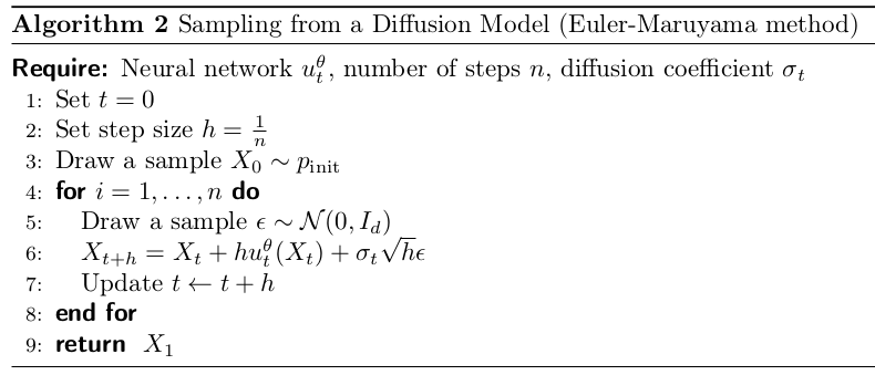

Constructing the Training Target

We have defined flow and diffusion models.

\[X_0 \sim p_{\text{init}}, \quad dX_t = u_t^\theta(X_t)\,dt \quad \text{(Flow model)}\] \[X_0 \sim p_{\text{init}}, \quad dX_t = u_t^\theta(X_t)\,dt + \sigma_t\,dW_t \quad \text{(Diffusion model)}\]

We have a neural network $u_t^\theta$ and we know how to sample from the resulting model. But we haven’t yet said how to train $u_t^\theta$ to actually produce data from $p_{\text{data}}$ rather than noise. Training requires a target to regress against.

The training objective is a mean-squared error:

\[\mathcal{L}(\theta) = \left\| u_t^\theta(x) - u_t^{\text{target}}(x) \right\|^2\]

The question is: what is $u_t^{\text{target}}$? It should be a vector field such that simulating the corresponding ODE actually converts $p_{\text{init}}$ into $p_{\text{data}}$. Deriving this requires three conceptual steps:

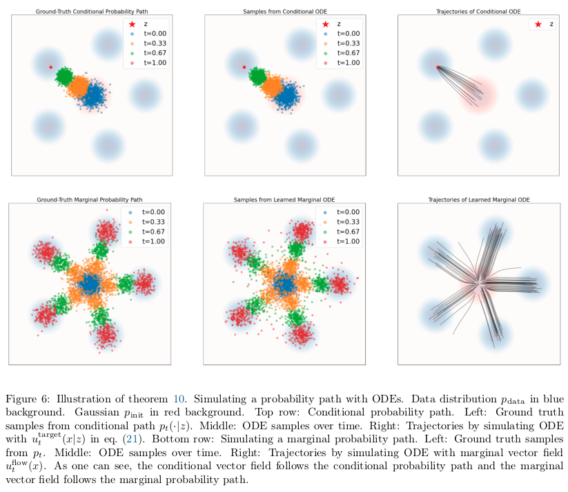
1. Define a probability path interpolating between $p_{\text{init}}$ and $p_{\text{data}}$
2. Construct a conditional vector field that generates each piece of that path
3. Average the conditional vector field over the data distribution to get the marginal vector field that generates the full path

Conditional and Marginal Probability Paths

What Is a Probability Path?

A probability path is a family of distributions ${p_t}{0 \leq t \leq 1}$ that interpolates smoothly from $p{\text{init}}$ to $p_{\text{data}}$. Think of it as a trajectory not in space $\mathbb{R}^d$, but in the space of distributions. At $t=0$, we have pure noise, and at $t=1$, we have data, and in between we have a gradual transition.

To construct such a path in a tractable way, we build it piece by piece, one data point at a time. For a single data point

\[z \in \mathbb{R}^d\]

we define a conditional (interpolating) probability path as a family of distributions $p_t(\cdot \mid z)$ satisfying:

Here, $\delta_z$ is the Dirac delta distribution: the simplest possible distribution, which always returns the single value $z$ when sampled.

A conditional probability path starts at the noise distribution $p_{\text{init}}$ and collapses to a sharp point mass at $z$ by time $t=1$. We want the distribution at the end of the process $p_1$ to be $\delta_z$. This means the model shouldn’t be fuzzy at the end, it should have arrived at one specific, clear data point $z$. The probability path $p_0(\cdot \mid z)$ is a mathematical way to transition from a wide, blurry Gaussian cloud at $t=0$ into this perfectly sharp Dirac spike at $t=1$.

As $t$ increases from 0 to 1, the distribution $x \sim p_t(\cdot \mid z)$ becomes more and more concentrated around $z$. At $t=1$, we have $x=z$ with certainty.

To obtain a noisy version of a data point $z$ at time $t$, we sample $x \sim p_t(\cdot \mid z)$. Although the conditional path is defined as going from noise (at $t=0$) to data (at $t=1$), sampling at a smaller $t$ produces noisier versions of $z$.

Some clarifications:

• $z$ is a full clean image: one training example sampled from the dataset, e.g. a crisp photo of a dog. It’s the same space $\mathbb{R}^{H \times W \times 3}$ as everything else.

• Sampling $x \sim p_t(\cdot \mid z)$ means: take that clean image $z$, and corrupt it to the noise level appropriate for time $t$. Concretely for the Gaussian path:

• At $t=0$: $x$ is pure noise $(\alpha_0=0)$. At $t=1$: $x=z$ exactly. In between: a blurry, noisy version of the dog photo.

The Marginal Probability Path

Each conditional path $p_t(\cdot \mid z)$ is anchored to a single data point $z$. To get a path that interpolates between the full noise distribution and the full data distribution, we marginalize over the data distribution:

Sampling from the marginal path $p_t$ is done in two steps: draw a data point, then draw a noisy version of it:

$p_t(x)$ is the distribution of noisy images produced by randomly choosing a data point and randomly corrupting it. It is not a procedure that tries to recreate the same $x$ from different $z$’s.

Difference between conditional and marginal probability paths:

• Conditional path: pick one specific training image (fix $z$), corrupt it differently each time (vary noise). All the noisy versions share the same underlying image $z$.
• Marginal path: pick a random training image (vary $z$) and corrupt it (vary noise). Now your noisy samples come from different underlying images too.

The marginal path is what you actually care about for generation because it reflects the full diversity of the dataset, not just one image.

The marginal path satisfies the boundary conditions automatically: because $p_t(\cdot \mid z) = p_{\text{init}}$ and because $p_t(\cdot \mid z) = \delta_z$, integratng against $p_{\text{data}}(z)$ gives $p_1 = p_{\text{data}}$. So:

\[p_0 = p_{\text{init}} \quad \text{and} \quad p_1 = p_{\text{data}}\]

There is a technical subtlety worth noting. We know how to sample from $p_t$ by using the two-step procedure above, but we don’t know the density values $p_t(x)$ at a specific point $x$ because the above integral is intractable. This distinction — tractable sampling, intractable density evaluation — will be crucial when we design the training algorithm.

Example: The Gaussian Conditional Probability Path

The most important example, which underlies all denoising diffusion models, is the Gaussian probability path. We introduce two noise schedulers:

\[\alpha_t, \beta_t : [0,1] \to \mathbb{R}\]

which are continuously differentiable, monotonic, and satisfy

\[\alpha_0 = \beta_1 = 0, \quad \alpha_1 = \beta_0 = 1\]

So,

\[\alpha_t = t, \quad \beta_t=1-t\]

The conditional probability path is defined as:

Checking the boundary conditions:

\[p_0(\cdot \mid z) = \mathcal{N}(\alpha_0 z, \beta_0^2 I_d) = \mathcal{N}(0, I_d) = p_{\text{init}}\] \[p_1(\cdot \mid z) = \mathcal{N}(\alpha_1 z, \beta_1^2 I_d) = \mathcal{N}(z, 0) = \delta_z\]

where the last step uses the fact that a Gaussian with zero variance and mean $z$ is the Dirac delta at $z$. Both boundary conditions are satisfied.

The Gaussian path has a particularly clean sampling procedure. To draw $x \sim p_t(\cdot \mid z)$:

This is a reparameterization: we can generate samples from $p_t(\cdot \mid z)$ by taking a clean data point $z$, scaling it by $\alpha_t$, and adding noise scaled by $\beta_t$. At $t=0$, the signal weight $\alpha_0=0$ and the noise weight $\beta_0=1$, so $x=\epsilon$ (pure noise). At $t=1$, $\alpha_1=1$ and $\beta_1=0$, so $x=z$ (pure data). In between, the image is a blend of data and noise.

Conditional and Marginal Vector Fields

The Central Problem

We’ve defined probability paths. Now we define a vector field, which is a function that assigns a velocity to every point in space at every time.

• Conditional vector field $u_t^{\text{target}}(x \mid z)$: the velocity field that moves a noisy image toward one specific clean image $z$. It knows the target destination.
• Marginal vector field $u_t^{\text{target}}(x)$: the velocity field that moves noisy images toward the full data distribution, without knowing which specific image $z$ they came from.

Now we need to find the marginal vector field $u_t^{\text{target}}$ such that the ODE:

\[dX_t = u_t^{\text{target}}(X_t)\,dt\]

with

\[X_0 \sim p_{\text{init}}\]

gives

\[X_t \sim p_t \quad \forall t \in [0,1]\]

and

\[X_1 \sim p_{\text{data}}\]

Computing the marginal vector field directly is intractable. The marginalization trick offers a way around this: find a conditional vector field that works for each individual data point $z$, then average appropriately.

The Marginalization Trick

For every data point $z \in \mathbb{R}^d$, let $u_t^{\text{target}}(x \mid z)$ be a conditional vector field such that simulating the corresponding ODE generates the conditional probability path:

Then the marginal vector field $u_t^{\text{target}}(x)$, defined by:

follows the marginal probability path:

In particular, $X_1 \sim p_{\text{data}}$, so the marginal vector field converts noise into data.

The above equation for marginal vector field is a weighted average of conditional vector fields. The weight $\frac{p_t(x \mid z)\, p_{\text{data}}(z)}{p_t(x)}$ is the posterior probability of data point $z$ given noisy observation $x$ at time $t$. This is Bayes’ theorem applied to the probability path. So intuitively, the marginal vector field at $x$ is the Bayes-weighted average of how each possible source $z$ would push $x$.

Target ODE for Gaussian Probability Paths

For the Gaussian path

\[p_t(\cdot \mid z) = \mathcal{N}(\alpha_t z, \beta_t^2 I_d)\]

there is a closed-form conditional vector field. Let:

\[\dot{\alpha}_t = \partial_t \alpha_t\] \[\dot{\beta}_t = \partial_t \beta_t\]

The conditional vector field is:

The intuition is that $u_t^{\text{target}}(x \mid z)$ must steer the distribution $p_t(\cdot \mid z) = \mathcal{N}(\alpha_t z, \beta_t^2 I_d)$ forward in time. The mean is moving at rate $\dot{\alpha}_tz$ and the spread is changing at a rate controlled by $\dot{\beta}_t$. The above formula encodes both effects.

Proof:

We construct the conditional flow $\psi_t^{\text{target}}(x \mid z)$ directly. We define:

\[\psi_t^{\text{target}}(x \mid z) = \alpha_t z + \beta_t x\]

The flow equation above linearly interpolates between pure noise (when $\beta_0=1, \alpha_0=0$) and the data point $z$ (when $\beta_1=0, \alpha_1=1$).

If $X_0 \sim p_{\text{init}} = \mathcal{N}(0, I_d)$, then:

\[X_t = \psi_t^{\text{target}}(X_0 \mid z) = \alpha_t z + \beta_t X_0 \sim \mathcal{N}(\alpha_t z, \beta_t^2 I_d) = p_t(\cdot \mid z)\]

So this flow does generate the conditional probability path.

It remains to extract the vector field from the flow. By the definition of a flow, we need

\[\frac{d}{dt}\,\psi_t^{\text{target}}(x \mid z) = u_t^{\text{target}}\big(\psi_t^{\text{target}}(x \mid z) \mid z\big)\]

Computing the left side:

\[\frac{d}{dt}(\alpha_t z + \beta_t x) = \dot{\alpha}_t z + \dot{\beta}_t x\]

Setting this equal to $u_t^{\text{target}}(\alpha_t z + \beta_t x \mid z)$ and solving for $u_t^{\text{target}}(x \mid z)$ by substituting

\[x \mapsto \frac{x - \alpha_t z}{\beta_t}\]

we get:

\[\dot{\alpha}_t z + \dot{\beta}_t \cdot \frac{x - \alpha_t z}{\beta_t} = u_t^{\text{target}}(x \mid z)\] \[\left(\dot{\alpha}_t - \frac{\dot{\beta}_t}{\beta_t}\alpha_t \right) z + \frac{\dot{\beta}_t}{\beta_t} x = u_t^{\text{target}}(x \mid z)\]

Conditional and Marginal Score Functions

Having constructed the training target for flow models (ODEs), we now extend to diffusion models (SDEs). The key new ingredient is the score function.

The Score Function

The marginal score function of $p_t$ is defined as:

This is the gradient of the log-density with respect to $x$. It is a vector field pointing in the direction of increasing probability: toward regions where $p_t$ is higher. Score functions are central to sampling methods (Langevin dynamics) and to diffusion model training.

Just as the marginal vector field could be expressed in terms of the conditional vector field, the marginal score can be expressed in terms of the conditional score function

This is the same weighted average structure as the marginalization trick for vector fields. The conditional score is tractable; the marginal score is not. But we can train a network to approximate the marginal score by regressing against the conditional score, just as for vector fields.

Score Function for Gaussian Probability Paths

For the Gaussian path

\[p_t(\cdot \mid z) = \mathcal{N}(\alpha_t z, \beta_t^2 I_d)\]

the conditional score is:

Proof of conditional score:

The Gaussian density is:

\[\mathcal{N}(x;\, \alpha_t z, \beta_t^2 I_d) = (2\pi \beta_t^2)^{-d/2} \exp\left(- \frac{\|x - \alpha_t z\|^2}{2\beta_t^2}\right)\]

Take the log:

\[\log \mathcal{N}(x;\, \alpha_t z, \beta_t^2 I_d) = -\frac{d}{2} \log(2\pi \beta_t^2) - \frac{\|x - \alpha_t z\|^2}{2\beta_t^2}\]

Take the gradient with respect to $x$ (first term vanishes as it is a constant in $x$):

\[\nabla_z \log \mathcal{N} = \nabla_z \left[ - \frac{\|x - \alpha_t z\|^2}{2\beta_t^2} \right]\]

Expand the numerator:

\[\|x - \alpha_t z\|^2 = (x - \alpha_t z)^{\top}(x - \alpha_t z)\] \[\nabla_z \|x - \alpha_t z\|^2 = 2(x - \alpha_t z)\] \[\nabla_z \log \mathcal{N} = - \frac{2(x - \alpha_t z)}{2\beta_t^2} = - \frac{x - \alpha_t z}{\beta_t^2}\]

The SDE Extension Trick

Using the same conditional and marginal vector fields $u_t^{\text{target}}(\cdot \mid z)$ and $u_t^{\text{target}}(\cdot)$ from before, and any diffusion coefficient $\sigma_t \ge 0$, we can construct an SDE that follows the same probability path:

In particular,

\[X_1 \sim p_{\text{data}}\]

The same holds with the conditional path and conditional vector field.

The extra term $\frac{\sigma_t^2}{2}\, \nabla \log p_t(X_t)$ is precisely what “corrects” the deterministic ODE drift to compensate for the noise added by the Brownian term $\sigma_t dW_t$. When $\sigma_t=0$, the SDE reduces to the ODE.

Summary: Derivation of the Training Target

For the flow model, the training target is the marginal vector field $u_t^{\text{target}}$. To construct it:

1. Choose a conditional probability path

   \[p_t(x \mid z)\]

   satisfying

   \[p_0(\cdot \mid z) = p_{\text{init}}\] \[p_1(\cdot \mid z) = \delta_z\]

2. Find a conditional vector field

   \[u_t^{\text{target}}(\cdot \mid z)\]

   such that

   \[\psi_t^{\text{target}}(X_0 \mid z) \sim p_t(\cdot \mid z)\]

   when

   \[X_0 \sim p_{\text{init}}\]

3. Define the marginal vector field by:

   \[u_t^{\text{target}}(x) = \int u_t^{\text{target}}(x \mid z)\, \frac{p_t(x \mid z)\, p_{\text{data}}(z)}{p_t(x)} \, dz\]

   This generates the marginal path:

   \[X_0 \sim p_{\text{init}}, \quad dX_t = u_t^{\text{target}}(X_t)\,dt \;\Longrightarrow\; X_t \sim p_t, \quad X_1 \sim p_{\text{data}}\]

   To extend to SDEs: for any $\sigma_t \ge 0$, the SDE

   \[X_0 \sim p_{\text{init}}, \quad dX_t = \left[ u_t^{\text{target}}(X_t) + \frac{\sigma_t^2}{2}\, \nabla \log p_t(X_t) \right] dt + \sigma_t\, dW_t\]

   also satisfies

   \[X_t \sim p_t\]

   where the marginal score function is:

   \[\nabla \log p_t(x) = \int \nabla \log p_t(x \mid z)\, \frac{p_t(x \mid z)\, p_{\text{data}}(z)}{p_t(x)} \, dz\]

For Gaussian Probability Path

The key formulas are:

\[p_t(x_\mid z) = \mathcal{N}(x;\, \alpha_t z, \beta_t^2 I_d)\] \[u_t^{\text{flow}}(x \mid z) = \left( \dot{\alpha}_t - \frac{\dot{\beta}_t}{\beta_t}\alpha_t \right) z + \frac{\dot{\beta}_t}{\beta_t} x\] \[\nabla \log p_t(x \mid z) = - \frac{x - \alpha_t z}{\beta_t^2}\]

for noise schedulers $\alpha_t, \beta_t \in \mathbb{R}$: continuously differentiable, monotonic functions such that $\alpha_0=\beta_1=0; \alpha_1=\beta_0=1$.

Training the Generative Model

We now have everything except the actual training procedure. We have defined flow and diffusion models, and we have derived the training target: the marginal vector field $u_t^{\text{target}}$ and marginal score $\nabla \log p_t$. The remaining question is: how do we train the neural network $u_t^\theta$ to approximate these targets?

The core challenge is that the marginal targets involve intractable integrals over all data points. The resolution is the central insight of this chapter: the intractable marginal loss and the tractable conditional loss have identical gradients, so minimizing the conditional loss is sufficient.

Flow Matching

Setting Up the Loss

We have a flow model:

\[X_0 \sim p_{\text{init}}, \quad dX_t = u_t^\theta(X_t)\,dt\]

We want

\[u_t^\theta \approx u_t^{\text{target}}\]

The natural loss is mean-squared error, averaged over time and over points sampled from the probability path. This is the flow matching (FM) loss:

Using the sampling procedure, we draw

\[z \sim p_{\text{data}}\]

then

\[x \sim p_t(\cdot \mid z)\]

This becomes:

Intuition: In words, this means sample a random time, pick a random training image, corrupt it to noise level $t$, evaluate the network, and penalize the squared distance from the marginal vector field target.

The problem computing $u_t^{\text{target}}$ requires the intractable integral:

\[u_t^{\text{target}}(x) = \int u_t^{\text{target}}(x \mid z)\, \frac{p_t(x \mid z)\, p_{\text{data}}(z)}{p_t(x)} \, dz\]

We cannot evaluate this during training.

The Conditional Flow Matching Loss

The fix is to replace the marginal vector field with the conditional one. Define the conditional flow matching (CFM) loss:

Since we have a closed-form formula for $u_t^{\text{target}}(x \mid z)$ , this is fully tractable.

The Fundamental Equivalence

The marginal and conditional flow matching losses differ only by a constant independent of $\theta$:

Minimizing $\mathcal{L}{\text{CFM}}$ via SGD is equivalent to minimizing $\mathcal{L}{\text{FM}}$. The minimizer $\theta^*$ satisfies

\[u_t^\theta = u_t^{\text{target}}\]

(given sufficient network expressivity).

Proof:

We start from $\mathcal{L}_{\text{FM}}$ and expand the squared norm using

\[\|a - b\|^2 = \|a\|^2 - 2 a^\top b + \|b\|^2\]

So we have:

\[\mathcal{L}_{\text{FM}}(\theta) = \mathbb{E}_{t,x \sim p_t} \big[ \|u_t^\theta(x)\|^2 \big] - 2\, \mathbb{E}_{t,x \sim p_t} \big[ u_t^\theta(x)^\top u_t^{\text{target}}(x) \big] + \underbrace{\mathbb{E}_{t,x \sim p_t} \big[ \|u_t^{\text{target}}(x)\|^2 \big]}_{=: C_1}\]

$C_1$ does not depend on $\theta$.

Now we rewrite the cross term. Using the sampling equivalence and plugging in the definition of $u_t^{\text{target}}(x)$:

\[\mathbb{E}_{t,x \sim p_t}\big[ u_t^\theta(x)^\top u_t^{\text{target}}(x) \big]\] \[= \int_0^1 \int p_t(x)\, u_t^\theta(x)^\top \left[ \int u_t^{\text{target}}(x \mid z)\, \frac{p_t(x \mid z)\, p_{\text{data}}(z)}{p_t(x)}\, dz \right] dx\, dt\] \[= \int_0^1 \int \int u_t^\theta(x)^\top u_t^{\text{target}}(x \mid z)\, p_t(x \mid z)\, p_{\text{data}}(z)\, dz\, dx\, dt\] \[= \mathbb{E}_{t, z \sim p_{\text{data}},\, x \sim p_t(\cdot \mid z)} \big[ u_t^\theta(x)^\top u_t^{\text{target}}(x \mid z) \big]\]

This is the crucial step: the marginal vector field inside the expectation is replaced by the conditional one. Substituting back:

\[\mathcal{L}_{\text{FM}}(\theta) = \mathbb{E}_{t, z, x} \left[ \|u_t^\theta(x)\|^2 - 2\, u_t^\theta(x)^\top u_t^{\text{target}}(x \mid z) \right] + C_1\]

Adding and subtracting $|u_t^{\text{target}}(x \mid z)|^2$ inside the expectation to complete the square:

\[= \mathbb{E}_{t,z,x} \left[ \|u_t^\theta(x) - u_t^{\text{target}}(x \mid z)\|^2 \right] + \underbrace{\mathbb{E}_{t,z,x}\left[-\|u_t^{\text{target}}(x \mid z)\|^2\right]}_{=: C_2} + C_1\] \[= \mathcal{L}_{\text{CFM}}(\theta) + \underbrace{C_1 + C_2}_{=: C}\]

Both $C_1$ and $C_2$ are independent of $\theta$, so $C$ is a constant. The gradients are therefore identical.

Flow Matching for Gaussian Conditional Probability Paths

For the specific choice

\[\alpha_t = t, \quad \beta_t = 1-t\]

We have

\[\dot{\alpha}_t = 1, \quad \dot{\beta}_t = -1\]

Conditional vector field:

\[u_t^{\text{target}}(x \mid z) = \left( \dot{\alpha}_t - \frac{\dot{\beta}_t}{\beta_t}\alpha_t \right) z + \frac{\dot{\beta}_t}{\beta_t} x\] \[u_t^{\text{target}}(x \mid z) = z - \epsilon\]

where

\[x = tz + (1-t)\epsilon\]

The CFM loss becomes:

Intuition: In words, this means sample a training image $z$, sample noise $\epsilon$, blend them into a noisy image $x$, and train the network to predict the direction from noise toward the clean image. This remarkably simple procedure is what underlies Stable Diffusion 3, Meta’s Movie Gen Video, and many other state-of-the-art models.

Flow Matching Training Algorithm

1. Sample a training image

   \[z \sim p_{\text{data}}\]

2. Sample time

   \[t \sim \text{Unif}[0,1]\]

3. Sample noise

   \[\epsilon \sim \mathcal{N}(0, I_d)\]

4. Set

   \[x = t z + (1 - t)\epsilon\]

5. Compute loss

   \[\mathcal{L}(\theta) = \|u_t^\theta(x) - (z - \epsilon)\|^2\]

6. Update $\theta$ via gradient descent

After training, generate samples by simulating the ODE.

The neural network $u_t^\theta$ takes the noisy image $x$ and time $t$ as input, outputs a velocity vector. During training, $x$ is sampled from the probability path and treated as a fixed input. Only $\theta$ is updated. The target velocity $(z-\epsilon)$ is computed analytically. No ODE is simulated during training.

Score Matching

Setting Up the Score Loss

We now extend from ODEs to SDEs. It has been shown before that the SDE follows the same probability path as the ODE is:

\[X_0 \sim p_{\text{init}}, \quad dX_t = \left[ u_t^{\text{target}}(X_t) + \frac{\sigma_t^2}{2}\, \nabla \log p_t(X_t) \right] dt + \sigma_t\, dW_t\]

To simulate this, we need to approximate the marginal score $\nabla \log p_t(x)$ with a score network

Exactly as before, we define two losses. The score matching (SM) loss:

This is intractable because $\nabla \log p_t(x)$ is intractable. The conditional score matching (CSM) loss:

This is tractable because we have a closed-form conditional score.

Equivalence for Score Matching

The score matching and conditional score matching losses differ by a constant:

Therefore:

\[\nabla_\theta \mathcal{L}_{\text{SM}}(\theta) = \nabla_\theta \mathcal{L}_{\text{CSM}}(\theta)\]

The minimizer $\theta^*$ satisfies

\[s_t^{\theta^*} = \nabla \log p_t\]

Proof:

The formula for $\nabla \log p_t(x)$ has exactly the same structure as the formula for $u_t^{\text{target}}(x)$: both are weighted averages of their conditional counterparts. The proof is therefore identical to that shown previously, replacing $u_t^{\text{target}}$ with $\nabla \log p_t$ throughout.

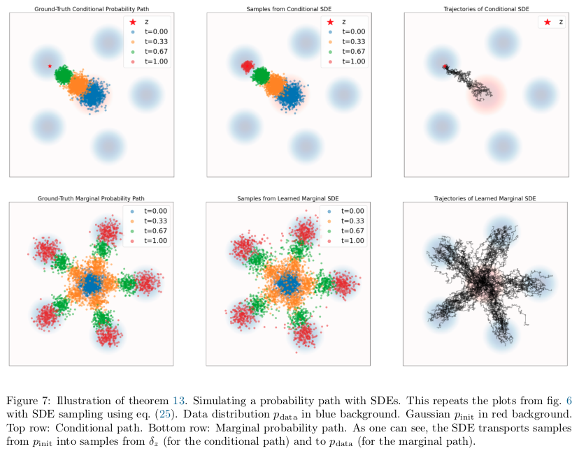
Training and Sampling a Diffusion Model

After training both $u_t^{\theta}$ and $s_t^\theta$ (or just one, since they can be converted and this will be shown below), we generate samples by simulating the SDE with any chosen $\sigma_t \ge 0$:

In theory, any $\sigma_t$ gives $X_1 \sim p_{\text{data}}$ under perfect training. In practice, numerical and training errors make some choices of $\sigma_t$ better than others. The optimal value must be found empirically.

Denoising Score Matching for Gaussian Paths

For the Gaussian path

\[p_t(x \mid z) = \mathcal{N}(\alpha_t z, \beta_t^2 I_d)\]

The conditional score is

\[\nabla \log p_t(x \mid z) = - \frac{x - \alpha_t z}{\beta_t^2}\]

Plugging into the CSM loss and using

\[x = \alpha_t z+\beta_t \epsilon\]

We have:

\[\mathcal{L}_{\text{CSM}}(\theta) = \mathbb{E}_{t,z,x \sim p_t(\cdot \mid z)} \left[ \left\| s_t^\theta(x) + \frac{x - \alpha_t z}{\beta_t^2} \right\|^2 \right]\] \[\mathcal{L}_{\text{CSM}}(\theta) = \mathbb{E}_{t,z,\epsilon \sim \mathcal{N}(0,I)} \left[ \left\| s_t^\theta(\alpha_t z + \beta_t \epsilon) + \frac{\epsilon}{\beta_t} \right\|^2 \right]\]

The score network $s_t^\theta$ is essentially learning to predict the noise $\epsilon$ used to corrupt the data point. This is why this loss is called denoising score matching.

The DDPM Noise Predictor Reparameterization

The loss above is numerically unstable when $\beta_t \approx 0$ (i.e. near $t=1$ where there is very little noise), because the $\frac{1}{\beta_t^2}$ factor blows up. The original DDPM paper proposed to drop this constant and reparameterize using a noise predictor network

\[\epsilon_t^\theta : \mathbb{R}^d \times [0,1] \to \mathbb{R}^d\]

via:

\[-\beta_t s_t^\theta(x) = \epsilon_t^\theta(x)\]

This gives the DDPM loss:

This is even simpler: corrupt a clean image with noise $\epsilon$, and train the network to predict that same noise back. The network learns to identify “what noise was added,” which implicitly encodes the direction toward the clean image.

Score Matching Training Algorithm for Gaussian Path

1. Sample

   \[z \sim p_{\text{data}}\]

2. Sample

   \[t \sim \text{Unif}[0,1]\]

3. Sample

   \[\epsilon \sim \mathcal{N}(0,I_d)\]

4. Set

   \[x_t = \alpha_t z + \beta_t \epsilon\]

5. Compute loss (either form):

   \[\mathcal{L}(\theta) = \left\| s_t^\theta(x_t) + \frac{\epsilon}{\beta_t} \right\|^2 \quad \text{or} \quad \mathcal{L}(\theta) = \left\| \epsilon_t^\theta(x_t) - \epsilon \right\|^2\]

6. Update $\theta$ via gradient descent

Conversion Between Vector Field and Score

For Gaussian paths, there is a remarkable bonus: learning either $u_t^\theta$ or $s_t^\theta$ gives you the other for free. The conversion formulas are:

Proof:

Starting from the conditional vector field:

\[u_t^{\text{target}}(x \mid z) = \left( \dot{\alpha}_t - \frac{\dot{\beta}_t}{\beta_t}\alpha_t \right) z + \frac{\dot{\beta}_t}{\beta_t} x\]

We substitute the conditional score:

\[\nabla \log p_t(x \mid z) = - \frac{x - \alpha_t z}{\beta_t^2}\]

So,

\[\alpha_t z = x + \beta_t^2 \nabla \log p_t(x \mid z)\] \[z = \frac{x + \beta_t^2 \nabla \log p_t(x \mid z)}{\alpha_t}\]

Substituting into the conditional vector field and simplifying algebraically:

\[u_t^{\text{target}}(x \mid z) = \left( \frac{\beta_t^2 \dot{\alpha}_t}{\alpha_t} - \dot{\beta}_t \beta_t \right) \nabla \log p_t(x \mid z) + \frac{\dot{\alpha}_t}{\alpha_t} x\]

Taking integrals (the same weighted average over $z$) on both sides, the conditional quantities become marginal ones:

\[u_t^{\text{target}}(x) = \left( \frac{\beta_t^2 \dot{\alpha}_t}{\alpha_t} - \dot{\beta}_t \beta_t \right) \nabla \log p_t(x) + \frac{\dot{\alpha}_t}{\alpha_t} x\] \[u_t^{\theta}(x) = \left( \frac{\beta_t^2 \dot{\alpha}_t}{\alpha_t} - \dot{\beta}_t \beta_t \right) s_t^\theta(x) + \frac{\dot{\alpha}_t}{\alpha_t} x\]

This means for Gaussian paths, there is no need to train $u_t^\theta$ and $s_t^\theta$ separately. You can choose either flow matching or score matching to train, then convert post-training. The denoising score matching loss and the conditional flow matching loss are in fact equal up to a constant in this case.

After training a score network $s_t^\theta$, sampling uses the SDE with arbitary $\sigma_t \ge 0$:

\[X_0 \sim p_{\text{init}}, \quad dX_t = \left[ \left( \frac{\beta_t^2 \dot{\alpha}_t}{\alpha_t} - \dot{\beta}_t \beta_t + \frac{\sigma_t^2}{2} \right) s_t^\theta(x) + \frac{\dot{\alpha}_t}{\alpha_t} x \right] dt + \sigma_t\, dW_t\]

This is stochastic sampling from a denoising diffusion model.

Summary: Training the Generative Model

Flow matching trains $u_t^\theta$ by minimizing the conditional flow matching loss:

After training, generate by simulating the ODE.

For diffusion models, additionally train a score network $s_t^\theta$ via denoising score matching:

Then generate by simulating the SDE with empirically chosen $\sigma_t \ge 0$:

For Gaussian paths specifically, the losses simplify to:

\[\mathcal{L}_{\text{CFM}}(\theta) = \mathbb{E}_{t,z,\epsilon} \left[ \left\| u_t^\theta(\alpha_t z + \beta_t \epsilon) - (\dot{\alpha}_t z + \dot{\beta}_t \epsilon) \right\|^2 \right]\] \[\mathcal{L}_{\text{CSM}}(\theta) = \mathbb{E}_{t,z,\epsilon} \left[ \left\| s_t^\theta(\alpha_t z + \beta_t \epsilon) + \frac{\epsilon}{\beta_t} \right\|^2 \right]\]

And the two networks convert into each other via:

\[u_t^{\theta}(x) = \left( \frac{\beta_t^2 \dot{\alpha}_t}{\alpha_t} - \dot{\beta}_t \beta_t \right) s_t^\theta(x) + \frac{\dot{\alpha}_t}{\alpha_t} x\]

So there is no need to train both separately. Denoising diffusion models are exactly this framework restricted to Gaussian probability paths.