Probabilistic Robotics

In progress

Resources

Programming

Basic Concepts of Probability

Terminology

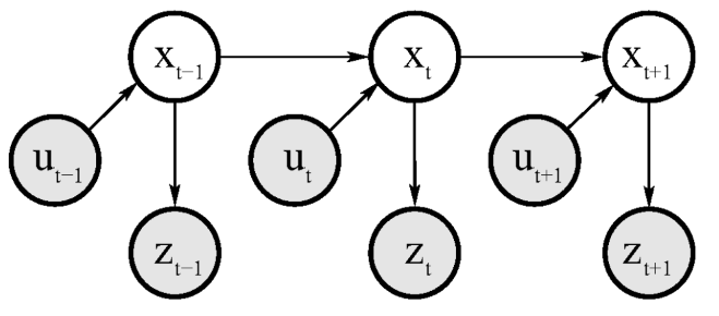
The environment, or world, is a dynamical system that possesses internal state. The robot can acquire information about its environment using its sensors. However, sensors are noisy, and there are usually many things that cannot be sensed directly. As a consequence, the robot maintains an internal belief with regards to the state of its environment.

State

• State - It is a collection of all aspects of the robot and its environment that can impact the future. Dynamic states are state variables that tend to change over time, while static states are non-changing. The state at time $t$ is denoted as $x_t.$
• Pose - The robot pose comprises of its location and orientation relative to a global reference frame. In the context of mobile robots, the pose is usually given by three variables, two location coordinates in the plane and one orientation w.r.t the vertical axis normal to the plane.
• The location and features of the surrounding objects in the environment are also state variables. Based on the quality of the state, robot environments can have even hundreds to billions of state variables.
• Some objects in the environment can be recognized reliably and are referred to as landmarks.
• Other state variables can include whether or not a sensor is broken, the level of battery charge, etc. These take discrete values.
• Markov chains - A state $x_t$ is said to be complete if the knowledge of past states, measurements or controls carry no additional information to help predict the future more accurately. The future may be stochastic but no variables prior to $x_t$ may influence the future states, unless this dependence is mediated through the state $x_t.$

Environment Interaction

• Sensor Measurements - Perception is the process by which the robot uses its sensors to obtain information about the state of its environment. Typically, sensor measurements have some delay and provide information about the state a few moments ago. However, we will assume that measurements corresponds to a specific point in time. Measurement data at point $t$ will be denoted by $z_t.$

  \[z_{t1:t2} = z_{t1},z_{t1+1},z_{t1+2},....,z_{t2}\]

• Control Actions - They carry information about the change of state of the environments and they change the state by actively asserting forces on the robot’s environment. It is denoted by $u_t.$

  \[u_{t1:t2} = u_{t1},u_{t1+1},u_{t1+2},....,u_{t2}\]

Hidden Markov Model

The emergence of state $x_t$ might be conditioned on all past states, measurements and controls. This gives us a probability distribution of the following form:

\[p(x_t | x_{0:t-1},z_{1:t-1},u_{1:t})\]

We assume that the robot executes the control action $u_1$ first and then takes the measurement $z_1$.

If the state $x$ is complete, then

\[p(x_t | x_{0:t-1},z_{1:t-1},u_{1:t}) = p(x_t|x_{t-1},u_t) \implies State \space transition \space probability\]

Similarly, if $x_t$ is complete, we have

\[p(z_t | x_{0:t},z_{1:t-1},u_{1:t}) = p(z_t|x_{t}) \implies Measurement \space probability\]

The state at time $t$ is stochastically dependent on the state at time $t-1$ and the control $u_t.$ The measurement $z_t$ depends stochastically on the state at time $t.$

Belief Distributions

Belief represents the robot’s internal knowledge about the state of the environment. We denote the belief over a state variable $x_t$ by $bel(x_t),$

\[bel(x_t) = p(x_t|z_{1:t},u_{1:t})\]

We assume that the belief is taken after incorporating the measurement $z_t$. Sometimes it is also useful to calculate the belief before incorporating $z_t$, just after executing $u_t.$

\[\bar{bel(x_t)} = p(x_t|z_{1:t-1},u_{1:t})\]

Calculating $bel(x_t)$ from $\bar{bel(x_t)}$ is called correction or measurement update.

Bayes Filter

Pseudo-code

Algorithm Bayes_filter ($bel(x_{t-1}),u_t,z_t):$

for all $x_t$ do:

\[\bar{bel(x_t)} = \int{p(x_t|u_t,x_{t-1}) bel(x_{t-1})dx_{t-1}}\] \[bel(x_t) = \eta p(z_t|x_t)\bar{bel(x_t)}\]

endfor

return $bel(x_t)$

Markov Assumption

Also called the complete state assumption, it postulates that the past and future data are independent if one knows the current state $x_t$. However, the following factors may have a systematic effect on sensor readings and induce violations to the Markov assumption:

• Unmodeled dynamics in the environment are not included in $x_t$
• Inaccuracies in probabilistic models - state transition probability and measurement probability
• Approximation errors when using approximate representations of belief functions
• Software variables in the robot control software that influence multiple controls

Estimation is after the occurrence of the event i.e. posterior probability. Prediction is a kind of estimation before the occurrence of the event i.e. apriori probability.

What is the difference between estimation and prediction?

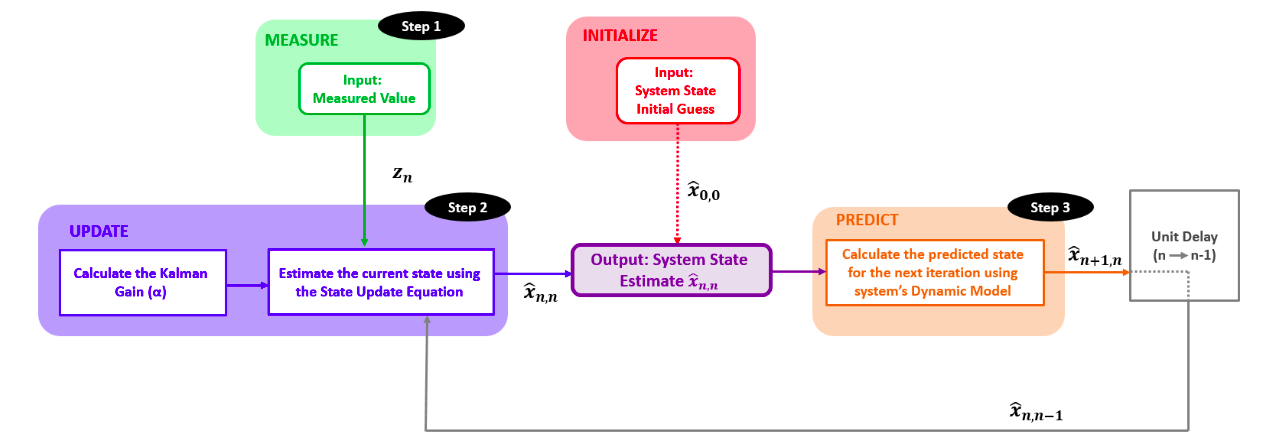
The $\alpha-\beta-\gamma$ Filter

Online Kalman Filter Tutorial

Notation

$x$ is the true value of the weight

$z_n$ is the measured value of the weight at time n

$\hat{x}_{n,n}$ is the estimate of $x$ at time n (the estimate is made after taking the measurement $z_n$)

\(\hat{x}_{n+1,n}\) is the estimate of the future state ( n+1 ) of $x$. The estimate is made at the time n. In other words, $\hat{x}_{n+1,n}$ is a predicted state or extrapolated state

\(\hat{x}_{n-1,n-1}\) is the estimate of xx at time n−1 (the estimate is made after taking the measurement $z_{n-1}$)

$\hat{x}_{n,n-1}$ is a prior prediction - the estimate of the state at time n. The estimate is made at the time n−1

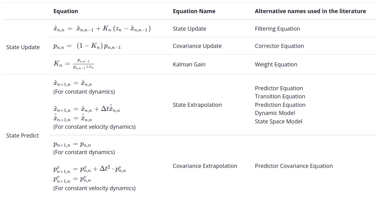
\[For \space constant \space dynamics: \newline \hat{x}_{n+1,n}= \hat{x}_{n,n}\] \[State \space Update \space Equation: \newline \hat{x}_{n,n} = \hat{x}_{n,n-1} + \alpha_n \left( z_{n} - \hat{x}_{n,n-1} \right)\]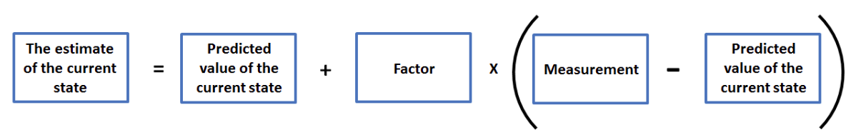

$\alpha_n$ is called the Kalman Gain

$(z_n - \hat{x}_{n,n-1})$  is the “measurement residual”, also called innovation. The innovation contains new information.

$\alpha - \beta$ Filter

\[State \space Extrapolation \space Equations: \newline\] \[x_{n+1}= x_{n}+ \Delta t\dot{x}_{n} \newline \dot{x}_{n+1}= \dot{x}_{n}\]

The above system of equations is also called Transition Equation or Prediction Equation, and is true for constant velocity dynamics.

$\alpha-\beta$ track update equations or $\alpha-\beta$ track filtering equations -

\[State \space Update \space Equation \space for \space position: \newline\] \[\hat{x}_{n,n} = \hat{x}_{n,n-1}+ \alpha \left( z_{n}- \hat{x}_{n,n-1} \right) \newline\] \[State \space Update \space Equation \space for \space velocity: \newline\] \[\hat{\dot{x}}_{n,n} = \hat{\dot{x}}_{n,n-1}+ \beta \left( \frac{z_{n}-\hat{x}_{n,n-1}}{ \Delta t} \right)\]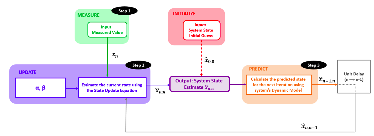

$\alpha-\beta-\gamma$ Filter

\[State \space Extrapolation \space Equations: \newline\] \[\hat{x}_{n+1,n}= \hat{x}_{n,n}+ \hat{\dot{x}}_{n,n} \Delta t+ \hat{\ddot{x}}_{n,n}\frac{ \Delta t^{2}}{2} \newline\] \[\hat{\dot{x}}_{n+1,n}= \hat{\dot{x}}_{n,n}+ \hat{\ddot{x}}_{n,n} \Delta t \newline\] \[\hat{\ddot{x}}_{n+1,n}= \hat{\ddot{x}}_{n,n}\] \[State \space Update \space Equations: \newline\] \[\hat{x}_{n,n}= \hat{x}_{n,n-1}+ \alpha \left( z_{n}- \hat{x}_{n,n-1} \right) \newline\] \[\hat{\dot{x}}_{n,n}= \hat{\dot{x}}_{n,n-1}+ \beta \left( \frac{z_{n}-\hat{x}_{n,n-1}}{ \Delta t} \right) \newline\] \[\hat{\ddot{x}}_{n,n}= \hat{\ddot{x}}_{n,n-1}+ \gamma \left( \frac{z_{n}-\hat{x}_{n,n-1}}{0.5 \Delta t^{2}} \right)\]

The main difference between these filters is the selection of weighting coefficients $\alpha-\beta-(\gamma)$. Some filter types use constant weighting coefficients; others compute weighting coefficients for every filter iteration (cycle).

The choice of the $\alpha,\beta,\gamma$ is crucial for proper functionality of the estimation algorithm.

Kalman Filter

Online Kalman Filter Tutorial

The Kalman Filter is an optimal filter. It combines the prior state estimate with the measurement in a way that minimizes the uncertainty of the current state estimate.

\[For \space constant \space dynamics: \newline p_{n+1,n}= p_{n,n}\] \[Covariance \space Extrapolation \space Equation: \newline p_{n+1,n}^{x}= p_{n,n}^{x} + \Delta t^{2} \cdot p_{n,n}^{v} \newline p_{n+1,n}^{v}= p_{n,n}^{v}\]

$p^x$ is the position estimate uncertainty, $p^v$ is the velocity estimate uncertainty, and the above is true for constant velocity dynamics.

Note that for any normally distributed random variable $x$ with variance ${\sigma}^2$, $kx$ is distributed normally with variance $k^2{\sigma}^2$, therefore the time term in the uncertainty extrapolation equation is squared.

\[\hat{x}_{n,n} = \hat{x}_{n,n-1} + \frac{p_{n,n-1}}{p_{n,n-1} + r_{n}}\left( z_{n} - \hat{x}_{n,n-1} \right)\]

Kalman Gain:

\[K_{n}= \frac{Uncertainty \quad in \quad Estimate}{Uncertainty \quad in \quad Estimate \quad + \quad Uncertainty \quad in \quad Measurement}= \frac{p_{n,n-1}}{p_{n,n-1}+r_{n}}\] \[0 \leq K_{n} \leq 1\] \[\left( 1 - K_{n} \right) = \left( 1 - \frac{p_{n,n-1}}{p_{n,n-1} + r_{n}} \right) = \left( \frac{p_{n,n-1} + r_{n} - p_{n,n-1}}{p_{n,n-1} + r_{n}} \right) = \left( \frac{r_{n}}{p_{n,n-1} + r_{n}} \right)\] \[Covariance \space Update \space Equation: \newline p_{n,n} = \left( 1 - K_{n} \right)p_{n,n-1}\]

This equation updates the estimate uncertainty of the current state. It is clear from the equation that the estimate uncertainty is constantly decreasing with each filter iteration, since $\left( 1-K_{n} \right) \leq 1$. When the measurement uncertainty is high, the Kalman gain is low. Therefore, the convergence of the estimate uncertainty would be slow. However, the Kalman gain is high when the measurement uncertainty is low. Therefore, the estimate uncertainty would quickly converge toward zero.

The Kalman Gain is close to zero when the measurement uncertainty is high and the estimate uncertainty is low. Hence we give significant weight to the estimate and a small weight to the measurement.

On the other hand, when the measurement uncertainty is low, and the estimate uncertainty is high, the Kalman Gain is close to one. Hence we give a low weight to the estimate and a significant weight to the measurement.

If the measurement uncertainty equals the estimate uncertainty, then the Kalman gain equals 0.5.

The Kalman Gain Defines the measurement’s weight and the prior estimate’s weight when forming a new estimate. It tells us how much the measurement changes the estimate.

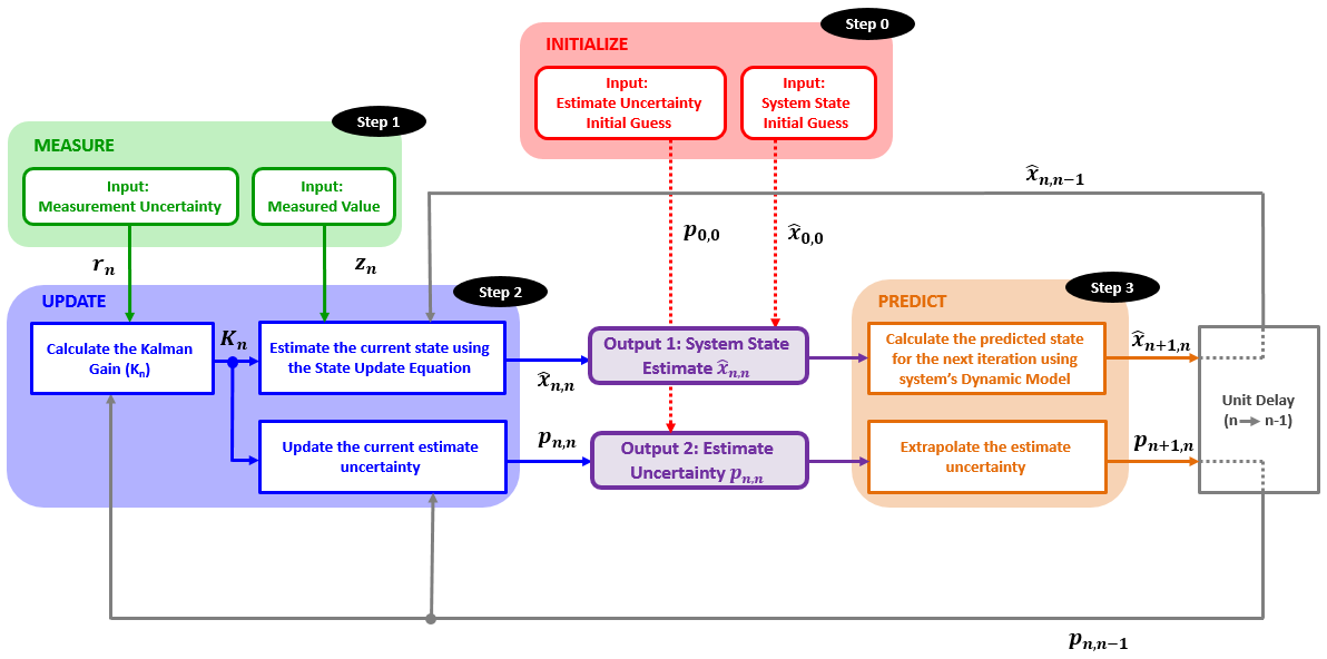
Summary of all 5 Kalman Equations

The State Extrapolation Equation and the Covariance Extrapolation Equation depend on the system dynamics.

SLAM

Localization

Navigation by odometry is prone to errors and can only give an estimate of the real pose of the robot. Further the robot moves, the larger is the error in the estimation of the pose. It can be compared to walking with eyes closed and counting our steps until we reach the destination. The further we walk with our eyes closed, the more uncertain we are about our location.

For moving short distances odometry is good enough, but when moving longer distances the robot must determine its position relative to an external reference called a landmark. This process is called localization.

Landmarks

Landmarks, such as lines on the ground or doors in a corridor can be detected and identified by the robot and used for localization.

Determining Position from Objects Whose Position Is Known

The following are two methods by which a robot can determine its position by measuring angles and distances to an object whose position is known.

From an Angle and a Distance

Suppose an object is placed at the origin $(x_0,y_0)$ of the coordinate system. The azimuth of the robot $\theta$ is the angle between the north and the forward direction of the robot. A laser scanner is used to measure the distance s from the object and the angle $\phi$ between the forward direction of the robot and the object.

\[\Delta x = s \sin(\theta-\phi) \newline \Delta y = s \cos(\theta-\phi)\]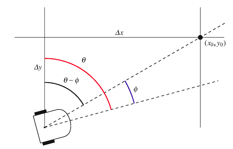

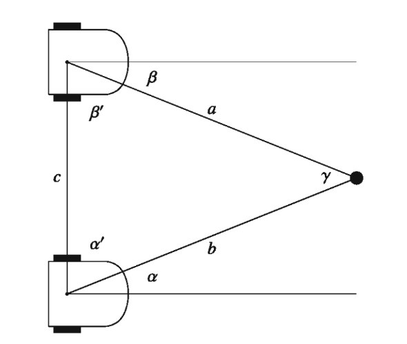
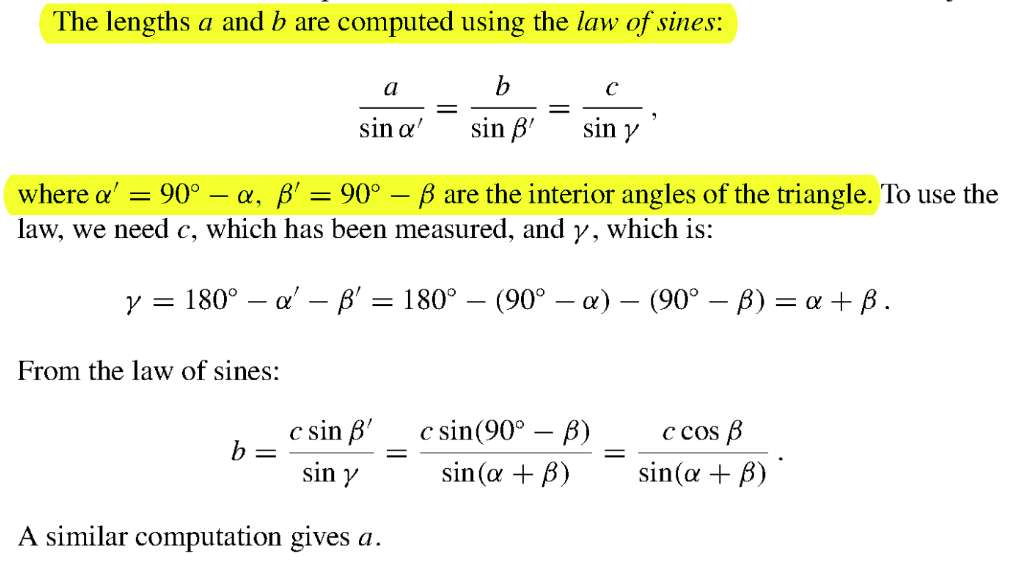
Triangulation

Triangulation is based on the principle that from two angles of a triangle and the length of the included side, the lengths of the other sides can be computed.

The robot measures the angles $\alpha$ and $\beta$ to the object from two positions separated by a distance $c$. This distance can be measured by odometry as the robot moves from one position to another, although this may be less accurate.

Global Positioning System

GPS navigation is based upon orbiting satellites. Each satellite knows its precise position in space and its local time. The position is sent to the satellite by ground stations and the time is measured by a highly accurate atomic clock on the satellite.

A GPS receiver must be able to receive data from 4 satellites. For this reason, a large number of satellites (24-32) is needed so that there is always a line-of-sight between any location and at least four satellites. From the time signals sent by a satellite, the distances from the satellites to the receiver can be computed by multiplying the times of travel by the speed of light. These distances and the known locations of the satellites enable the computation of the three-dimensional position of the receiver: latitude, longitude and elevation.

Advantages:

• Accurate
• Easily available - require only an electronic component which is small and inexpensive

Disadvantages:

• Positional error is roughly 10m. Not sufficient to perform tasks that need higher accuracy.
• GPS signals are not strong enough for indoor navigation and are subject to interference in dense urban environments.

Probabilistic Localization

• Consider a robot that is navigating within a known environment for which it has a map.
• Suppose the map shows 5 doors (dark gray) and 3 areas where there is no door (light gray). The task of the robot is to enter a specific door.
• By odometry, the robot can determine its current position given a known starting position.

Mapping

A robot can use its capability to detect objects to localize itself, and this information is usually provided by a map. However, building a map requires the robot to localize itself, but at the same time, solving the localization problem requires a map. Hence, we are now presented with a chicken-and-egg problem. This problem is overcome by using SLAM algorithms.

Discrete and Continuous Maps

A robot requires a non-visual representation of a map that it can store in its memory. There are 2 techniques for storing maps: discrete maps (or grid maps) and continuous maps.

Sonar Sensor Model

Frontier Algorithm

Mapping using Knowledge of the Environment

Even with bad odometry, the robot can construct a better map if it has some information on the structure of the environment. Suppose that the robot tries to construct the plan of a room by following its walls. If the robot knows in advance that the walls are straight and perpendicular to each other, the robot can correctly construct the map.

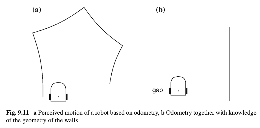
There will also be an error when measuring the lengths of the walls and this can lead to the gap shown in the figure between the first and the last walls. If the robot is mapping a large area, the problem of closing a loop in a map is hard to solve because the robot has only a local view of the environment.

Map correction can be improved by using sensor data that can give information on regular features in the environment. The regular features can be lines on the ground, a global orientation, or the detection of features that overlap with other measurements.

Large area measurements facilitate identifying overlaps between the local maps that are constructed at each location as the robot moves through the environment. By comparing local maps, the localization can be corrected and the map can be updated accurately.

SLAM Perception

Due to odometry and perception error, there is a mismatch between the current map and the sensor data which should correspond to the known part of the map.

How is this mismatch corrected?

• We assume that the odometry does give a reasonable estimation of the pose of the robot.
• For each relatively small possible error in the pose, we compute what the perception of the current map would be and compare it with the actual perception computed from the sensor data.
• The pose that gives the best match is chosen as the actual pose of the robot and the current map is updated accordingly.

The similarity matrix is computed, and once we have this result, we correct the pose of the robot and use data from the perception map to update the current map stored in the robot’s memory.

Probabilistic SLAM

The SLAM problem asks if it is possible for a mobile robot to be placed at an unknown location in an unknown environment and for the robot to incrementally build a consistent map of this environment while simultaneously determining its location within this map.

Both the trajectory of the platform and the location of all landmarks are estimated on-line without the need for any a priori knowledge of location.

SLAM problems possess a continuous and a discrete component:

• Continuous estimation problem: Deals with location of the objects in the map and the robot’s own pose variables.
• Discrete estimation problem: Deals with correspondence, i.e., the relation of the object to previously detected objects. The reasoning is discrete - whether the object is same as a previously detected object or not.

Online SLAM: Involves estimating the posterior over the momentary pose along with the map.

\[p(x_t,m | z_{1:t}, u_{1:t})\]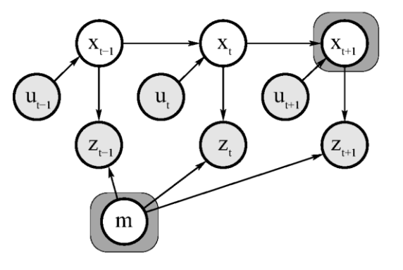

Full SLAM: Involves calculating the posterior over the entire path along with the map, instead of just the current pose.

\[p(x_{1:t},m | z_{1:t}, u_{1:t})\]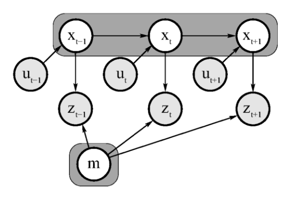

The online SLAM problem is the result of integrating out past poses from the full SLAM problem:

\[p\left(x_t, m \mid z_{1: t}, u_{1: t}\right)=\iint \cdots \int p\left(x_{1: t}, m \mid z_{1: t}, u_{1: t}\right) d x_1 d x_2 \ldots d x_{t-1}\]

Solving the SLAM problem requires that a state transition model and an observation model be defined describing the effect of the control input and observation respectively.

• The observation model describes the probability of making an observation \(z_k\) when the vehicle location and landmark locations are known $$ P(z_k

  x_k,m) $$.

• The motion model for the vehicle described in terms of a probability distribution on state transitions $$ P(x_k

  x_{k-1},u_k) $$.

The SLAM algorithm is now implemented in a recursive (sequential) prediction (time-update) correction (measurement-update) form.

Time update:

\[\begin{aligned}& P\left(\mathbf{x}_k, \mathbf{m} \mid \mathbf{Z}_{0: k-1}, \mathbf{U}_{0: k}, \mathbf{x}_0\right) \\& =\int P\left(\mathbf{x}_k \mid \mathbf{x}_{k-1}, \mathbf{u}_k\right) \times P\left(\mathbf{x}_{k-1}, \mathbf{m} \mid \mathbf{Z}_{0: k-1}, \mathbf{U}_{0: k-1}, \mathbf{x}_0\right) \mathrm{d} \mathbf{x}_{k-1}\end{aligned}\]

Measurement update:

\[\begin{aligned}& P\left(\mathbf{x}_k, \mathbf{m} \mid \mathbf{Z}_{0: k}, \mathbf{U}_{0: k}, \mathbf{x}_0\right) \\& =\frac{P\left(\mathbf{z}_k \mid \mathbf{x}_k, \mathbf{m}\right) P\left(\mathbf{x}_k, \mathbf{m} \mid \mathbf{Z}_{0: k-1}, \mathbf{U}_{0: k}, \mathbf{x}_0\right)}{P\left(\mathbf{z}_k \mid \mathbf{Z}_{0: k-1}, \mathbf{U}_{0: k}\right)}\end{aligned}\]

EKF SLAM

EKF-SLAM (Cyrill Stachniss)

It takes in observed landmarks from the environment and compares them with the known landmarks to find associations and new landmarks. It then uses the association to correct the state and state covariance matricies.

Maps in EKF SLAM are feature-based, which means they are composed of point landmarks. It tends to work well the less ambiguous the landmarks are, and hence requires significant engineering of feature detectors, sometimes using artificial beacons as features.

EKF SLAM makes a Gaussian noise assumption for robot motion and perception.

SLAM with Known Correspondence

It addresses only the continuous portion of the SLAM problem. In addition to estimating the robot pose, the algorithm also estimates the coordinates of all landmarks encountered along the way.

Let the combined state vector comprising the robot pose and the map be denoted by $y_t$.

\[\begin{aligned}& y_t=\left(\begin{array}{l}x_t \\m\end{array}\right) \\& =\left(\begin{array}{llllllllllll}x & y & \theta & m_{1, x} & m_{1, y} & s_1 & m_{2, x} & m_{2, y} & s_2 & \ldots & m_{N, x} & m_{N, y} & s_N\end{array}\right)^T \\&\end{aligned}\]

where $x,y,\theta$ denote the robot’s coordinates at time t.$m_{i,x},m_{i,y}$ are the coordinates of the i-th landmark for i=1,2,…,N and $s_i$ is its signature. The dimension of this state vector is 3N+3, where N is the number of landmarks.

Extended Kalman Filter Algorithm

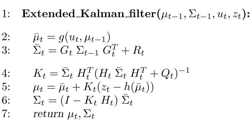
Inputs to the above algorithm are - the corrected estimate from the previous iteration, covariance or uncertainties, control input and measurements.

Line 2 represents the motion model. Line 4 is calculating the Kalman Gain. Lines 5 and 6 are the update equations.

Disadvantages of EKF SLAM:

• Linearization errors: The EKF SLAM algorithm relies on linearizing the nonlinear motion and measurement models, which can lead to approximation errors. These errors can accumulate over time, leading to inaccurate state estimates.
• Computational complexity: EKF SLAM is computationally intensive, and its complexity grows with the number of landmarks and the size of the state vector. This can make it difficult to use in real-time applications or on resource-limited devices.
• Limited observability: EKF SLAM assumes that all landmarks are observable, but in practice, this may not be the case. Landmarks that are not observed cannot be included in the state estimate, which can lead to inaccuracies.
• Sensitivity to initialization: The EKF SLAM algorithm is sensitive to the initial estimates of the robot’s pose and the landmark locations. Poor initial estimates can result in the algorithm converging to the wrong solution or getting stuck in a local minimum.
• Difficulty in handling loop closures: EKF SLAM assumes that the robot’s path is acyclic, which means it cannot handle loop closures. Loop closures occur when the robot revisits a previously visited location, and they are essential for accurate mapping. Handling loop closures requires more complex algorithms such as GraphSLAM.

Loop Closing

In loop closing, the SLAM algorithm attempts to identify and correct errors in the estimated robot trajectory by detecting and closing loops in the generated map. A loop is created when the robot revisits a previously mapped location after having moved through some other parts of the environment. When a loop is detected, the SLAM algorithm tries to reconcile the previously mapped location with the current robot pose estimate, usually by optimizing the robot’s trajectory using bundle adjustment or similar techniques.

Loop closing is important in SLAM because it enables the creation of consistent and accurate maps of the environment. Without loop closing, SLAM algorithms can suffer from drift, in which errors accumulate over time, causing the estimated robot pose to diverge from the true pose. Loop closing helps to correct such errors and ensure that the generated map is globally consistent.

• Loop closing means revisiting and recognizing an already mapped area. It reduces uncertainty in robot and landmark estimates.
• Uncertainties collapse after a loop closure, whether the closure was correct or not.
• This can be exploited when exploring an environment for the sake of better and more accurate maps.
• However, wrong loop closures lead to filter divergence.

GraphSLAM

Graph-based SLAM using Pose Graphs (Cyrill Stachniss)

GraphSLAM extracts from the data a set of soft constraints represented by a sparse graph. It obtains the map and the robot path by resolving these constraints into a globally consistent estimate.

The constraints are generally nonlinear, but in the process of resolving them they are linearized and transformed into an information matrix.

Each edge in the graph corresponds to an event: a motion event generates an edge between two robot poses, and a measurement event creates a link between a pose and a feature in the map.

For a linear system, these constraints are equivalent to entries in an information matrix and an information vector of a large system of equations.

Adding Confidence Measures

• Linear Least Squares allows us to include a weighting of each linear constraint.
• If we know something about how confident a measure is, we can include that in the computation.
• We weight each constraint by a diagonal matrix where the weights are 1/(variance for each constraint).
• Highly confident constraints have low variance; 1/variance is large weight, and vice-versa.

Cyclic Dependence

• Features that are observed multiple times, with large time delays in between.
• This might be the case because the robot goes back and forth through a corridor, or because the world possesses cycles.
• In either situation, there will exist features that are seen at drastically different time steps.