Development of Python-Based Simulator for Analyzing Autonomous Underwater Glider Motions and Performance

The following project was done as part of my undergraduate thesis at the Institute for Systems and Robotics, Lisbon under the supervision of Dr. David Cabecinhas and Dr. Pedro Batista

Abstract

The objective of this thesis is to design, develop, and implement a comprehensive Python-based simulator for Autonomous Underwater Gliders (AUGs), enabling the precise simulation and in-depth analysis of various motions exhibited by them. Underwater Gliders are a unique kind of vehicle that fall under the class of Autonomous Underwater Vehicles (AUVs), which maneuver through a water body by varying their buoyancy and attitude using internal mass actuators and a buoyancy engine.

The simulator will be used in analyzing the dynamics and behaviors of various glider models, such as the Slocum, Spray, and Rogue, both in a simplified two dimensional setting, as well as in full three dimensional gliding. Marine researchers can configure the simulator to specific mission scenarios and for specific glider designs.

The development of such a robust platform will serve as a valuable resource for researchers and practitioners in the field of marine robotics by facilitating the examination and evaluation of different motion patterns. This enhances our understanding of AUG behavior and performance, thereby furthering the development of such vehicles.

Introduction

Autonomous Underwater Gliders

Autonomous Underwater Gliders (AUGs) are a class of underwater robots that fall under the category of Autonomous Underwater Vehicles (AUVs). Unlike traditional propeller-driven vehicles that use external thrusters to move, AUGs are set apart because of their reliance on buoyancy-driven propulsion systems. This unique feature enables these gliders to achieve sustained vertical movement through the water column by harnessing changes in buoyancy and hydrodynamic forces.

Design

The design of AUGs can vary slightly depending on the models and the applications that they serve. However, most of them have a cylindrical hull, and are roughly shaped like a torpedo. They are typically small and reusable vehicles, with a weight of around 50 kg and 2m length, making them suitable for small missions and easily operated by fewer people. They are capable of operating at low speeds of 20-30 cm/s and can traverse thousands of kilometers over several months.

Several AUG models have been developed over the past years, such as the Slocum, Spray, and Seaglider. Each of these AUG models have slightly different design approaches, including battery and thermal powered propulsion, speed and depth capabilities, strategies to reduce drag, wing spans, and communication methods. Despite these differences, all of them have some standard dynamic characteristics, which will be discussed in Chapter 3.

Applications

Some of the applications of AUGs include:

• Study of ocean currents - Equipped with various sensors, AUGs can collect data on water temperature, salanity, and other parameters to better understand the patterns of ocean currents. They can also measure the levels of dissolved oxygen, pH, and other nutrients to assess the health of marine ecosystems.
• Climate change - They can help in predicting the rise in sea level due to the melting of polar ice caps, and can also monitor the levels of carbon dioxide in the water.
• Defense - AUGs can be used by the military/Navy for monitoring underwater activities, locate sea mines, and carry out secret missions.
• Disaster management - They can be used to detect changes in the oceans, such as temperature, vibrations in the sea floor that may indicate the occurrence of a tsunami or a hurricane.

Motivation

The development of a simulator for AUGs would help researchers to assess glider behavior under various conditions, validate algorithms, and conduct virtual missions.

Need for a Simulator

The use of AUGs has become increasingly important in the field of oceanography due to their exceptional efficiency and adaptability in collecting valuable data. These underwater vehicles are designed to independently navigate the ocean, carrying out various missions ranging from oceanographic data collection to environmental monitoring. This makes them essential assets for understanding and addressing critical challenges in marine science and technology.

Despite their growing importance in marine research and exploration, a noticeable shortage of accessible simulators specifically for the analysis and testing of underwater gliders persists. This glaring gap in available simulation tools presents a significant challenge to researchers and engineers in the field. The absence of user-friendly, open-source simulators severely limits our ability to comprehensively study and validate glider behaviors.

The analysis of the dynamics of AUGs is a highly sophisticated and challenging task. The core features may differ for different glider models, which can influence the dynamics and behaviors of the AUG, such as different mechanisms for internal mass actuation and ballast systems, use of external rudders, etc. This necessitates the need for a robust simulator that can be easily tailored to different AUG models depending on their application.

In the future, the use of a simulator can contribute to the development of methods for improved performance in specific flight regimes, as well as the testing of novel flight trajectories, optimization of control algorithms, and conducting virtual experiments. In addition, the simulator can allow for the comparison of performance of glider models such as the Slocum, Spray, and Seaglider.

Thus, this thesis aims to address this pressing need by developing an open-source simulator specifically for AUGs, thereby paving the way for the development of more efficient and advanced glider technologies.

Existing Underwater Simulators

While there do exist some underwater simulators, specifically for Autonomous Underwater Vehicles (AUVs), they are either not very suitable for AUGs, not very efficient, or not open-source.

Every AUG model, such as the Slocum, and Spray, comes with a “Simulation” option that can help in planning missions. This however, carries out simulations in real-time, due to which a simulation to plan missions for a week will take a week to run.

The following are a few existing open-source simulators:

DAVE

DAVE Aquatic Virtual Environment (DAVE) is a specialized simulation platform built on ROS and Gazebo, and is designed for the testing of underwater robots. It focuses on autonomous underwater vehicles (AUVs/UUVs) and their ability to carry out missions involving tasks like autonomous manipulation.

With ROS being widely used among the robotics community, this simulator offers great functionality and robustness. However, it is based on the kinematic model of an AUG, which is not very reliable. Interfacing the physical glider’s simulation API with ROS is also a challenging task. Moreover, reading the glider data, such as position of center of mass, variation of internal mass actuators, etc. is not straightforward to do. Additionally, changing the glider model, or its system dynamics is tedious, which necessitates the need for a more simple and efficient simulator.

Github: DAVE Simulator

WAVE

The WAVE simulator is a MATLAB based simulator that can be used to evaluate and improve the performance of an AUV by varying the blade geometry and braking strategies of the arms. It can be used in the development and testing of wing profiles and braking strategies.

Github: WAVE Simulator

FISH GYM

Fish Gym is a physics-based simulation platform particularly for bionic underwater robots. It is integrated into the OpenAI Gym interface, thereby enabling the use of reinforcement learning algorithms and control techniques on the underwater agents.

Underlying Principles of Glider Behavior

As mentioned in Fossen’s “Guidance and Control of Ocean Vehicles”, the modeling of marine vehicles requires the study of statics and dynamics. Statics deals with the equilibrium of bodies, i.e., bodies at rest or moving with constant velocity. Dynamics is concerned with bodies having accelerated motion. Dynamics, in turn, is divided into Kinematics and Kinetics. Kinematics treats only the geometrical aspects of motion, and Kinetics is the analysis of forces that cause this motion.

The overall kinematics and dynamics of AUGs are derived below, and the model presented here follows the glider model presented by Graver.

Kinematics

Defining two separate frames of reference makes it easier to model an AUG having 6 Degrees of Freedom (DOF). These are:

Inertial Frame

The Inertial Frame serves as a global reference frame, as it is fixed to the surface of the Earth. This frame lets us understand the position of the glider relative to the Earth, enabling precise navigation and global planning. The accelerations of a point on the Earth’s surface can be neglected since the motion of the Earth hardly affects low speed marine vehicles.

Let $xyz$ be the fixed inertial frame, such that the $x$ and $y$ axes lie in the horizontal plane, perpendicular to gravity. The $z$ axis points downward in the direction of gravity and denotes depth. The frame can be chosen on the surface of the water body such that $z = 0$.

Body-Fixed Frame

The Body-Fixed Frame is attached to the glider’s body and moves along with it. It allows for measuring the internal dynamics of the glider, and control inputs. This local reference is vital for precise maneuvers and simplifying how we gather information from the on-board sensors.

The Origin $O$ of the body-fixed frame usually coincides with the vehicle’s Center of Buoyancy (CoB). The body axes $X_{0}$, $Y_{0}$, $Z_{0}$ coincide with the principal axes of inertia:

• $X_{0}$ is the longitudinal axis - from aft to fore
• $Y_{0}$ is the transverse axis - directed to the starboard
• $Z_{0}$ is the normal axis - from top to bottom

The general motion of an AUG in 6 DOF can be described by the following vectors:

\[\begin{align}{\boldsymbol{\eta}=[\boldsymbol{b}^T,\boldsymbol{\eta_2}^T]^{T};\ \ \ \boldsymbol{b}=[x,y,z]^{T};\ \ \ \boldsymbol{\eta_2}=[\phi,\theta,\psi]^{T}}\\ {\boldsymbol{\nu}=[\boldsymbol{\nu}^{T},\boldsymbol{\Omega}^{T}]^{T};\ \ \ \boldsymbol{v}=[v_1,v_2,v_3]^{T};\ \ \boldsymbol{\Omega}=[\Omega_1,\Omega_2,\Omega_3]^{T}}\\ {\boldsymbol{\tau}=[\boldsymbol{\tau_{1}}^{T},\boldsymbol{\tau_{2}}^{T}]^{T};\ \ \ \boldsymbol{\tau_1}=[X, Y, Z]^{T};\ \ \ \boldsymbol{\tau_{2}}=[K,M,N]^{T}}\end{align}\]

Where $\boldsymbol{\eta}$ is the position and orientation in the inertial frame, $\boldsymbol{\nu}$ is the linear and angular velocity in the body-fixed frame, and $\boldsymbol{\tau}$ is the force and moment in the body-fixed frame.

The body-fixed frame can be related to the earth-fixed frame with the linear velocity and angular velocity transformations, using the Euler angles: roll ($\phi$), pitch ($\theta$), and yaw ($\psi)$.

The vehicle’s vectors in the inertial frame is given by the velocity transformation:

\[\begin{align} \boldsymbol{\dot{b}={J}_{1}({\eta}_{2})v} \end{align}\]

Where \({J}_{1}({\eta}_{2})\) is the transformation matrix. For simple principal rotations,

\[\begin{align} \boldsymbol{J_1\left(\eta_2\right)}=\left[\begin{array}{ccc} \mathrm{c} \psi \mathrm{c} \theta & -\mathrm{s} \psi \mathrm{c} \phi+\mathrm{c} \psi \mathrm{s} \theta \mathrm{s} \phi & \mathrm{s} \psi \mathrm{s} \phi+\mathrm{c} \psi \mathrm{c} \phi \mathrm{s} \theta \\ \mathrm{s} \psi \mathrm{c} \theta & \mathrm{c} \psi \mathrm{c} \phi+\mathrm{s} \phi \mathrm{s} \theta \mathrm{s} \psi & -\mathrm{c} \psi \mathrm{s} \phi+\mathrm{s} \theta \mathrm{s} \psi \mathrm{c} \phi \\ -\mathrm{s} \theta & \mathrm{c} \theta \mathrm{c} \phi & \mathrm{c} \theta \mathrm{c} \phi \end{array}\right] \end{align}\]

The angular velocity transformation is given by

\[\begin{align} \boldsymbol{\dot{\eta}_2=J_2\left(\eta_2\right) \Omega} \end{align}\] \[\begin{align} \boldsymbol{J_2\left(\eta_2\right)}=\left[\begin{array}{ccc} 1 & s \phi \mathrm{t} \theta & c \phi \mathrm{t} \theta \\ 0 & c \phi & -s \phi \\ 0 & s \phi / c \theta & c \phi / c \theta \end{array}\right] \end{align}\]

Thus, the kinematic equations can be expressed in the vector form as

\[\begin{align} \left[\begin{array}{c} \boldsymbol{\dot{b}} \\ \boldsymbol{\dot{\eta}_2} \end{array}\right]=\left[\begin{array}{cc} \boldsymbol{J_1\left(\eta_2\right)} & \boldsymbol{0_{3 \times 3}} \\ \boldsymbol{0_{3 \times 3}} & \boldsymbol{J_2\left(\eta_2\right)} \end{array}\right]\left[\begin{array}{c} \boldsymbol{v} \\ \boldsymbol{\Omega} \end{array}\right] \end{align}\]

Since we use \(\boldsymbol{J_{1}(\eta_{2})}\) very often, we replace this rotation matrix with $\boldsymbol{R}$ to map vectors expressed in the body frame to the inertial frame.

Vehicle Model

The underwater glider is considered to be a rigid body fitted with hydrofoils, which are underwater wings that allow it to glide forward, and a tail. The glider dynamics are derived by considering the entire frame to be immersed in a fluid.

The glider comprises of the following masses:

• The hull mass $m_{h}$, which is fixed and uniformly distributed throughout the body.
• The ballast mass $m_{b}$ which varies as water is pumped in and out of the system, and whose position is fixed with respect to the vehicle’s CoB.
• The internal moving mass $\bar{m}$ which moves inside the glider’s body but has a fixed mass.
• The static offset mass $m_{w}$ which is a fixed point mass that can be offset from the vehicle’s CoB.

The stationary mass of the glider is given by \begin{align} m_{s} = m_{h} + m_{b} + m_{w} \end{align}

The total mass of the vehicle is then \begin{align} m_{t} = m_{h} + m_{b} + m_{w} + \bar{m} = m_{s} + \bar{m} \end{align}

The positions of the internal point masses $m_{b}$ and $m_{w}$ inside the glider frame is given by the vectors $\boldsymbol{r_{b}}$ and $\boldsymbol{r_{w}}$ with respect to the Center of Buoyancy (CoB). The vector $\boldsymbol{r_{p}(t)}$ gives the position of the movable mass $\bar{m}$ in the body-fixed frame.

The ballast mass $m_{b}$ changes as water is pumped in or emptied off of the buoyancy compartments in order to vary the vehicle’s buoyancy. The movable mass $\bar{m}$ is used to vary the pitch of the glider, which together with the ballast mass $m_{b}$ helps the glider maneuver. The offset static point mass $m_{w}$ can be set to balance the rolling and pitching moment on the glider at equilibrium.

We denote $m$ to be the mass of fluid displaced by the glider. As a result, the net buoyancy is given by \begin{align} m_{0} = m_{t} - m \end{align}

When $m_{0}$ is positive, it means that the vehicle is negatively buoyant (it sinks), and similarly, when $m_{0}$ is negative, it means that the vehicle is positively buoyant (it floats).

Ballast System and Controlled Masses

The ballast system is responsible for varying the AUGs depth within the water column. It comprises of volume compartments that can be flooded or emptied with water to change the glider’s buoyancy. By doing so, the glider can achieve positive, negative, or neutral buoyancy, and can either ascend or descend.

• Positive buoyancy - glider floats upward
• Negative buoyancy - glider sinks downward
• Neutral buoyancy - glider neither floats nor sinks

The type of ballast system used and its position inside the glider is motivated by the geometrical design of the AUG model. For most this thesis we model the Slocum glider, in which the ballast mass $m_{b}$ and internal moving mass $\bar{m}$ are both well forward of the glider’s CoB. The Slocum design uses a syringe-type ballast tank to take in or pump out water.

An important control input for the ballast mass is the ballast pumping rate $\dot{m_{b}}$. We assume that when ballast is pumped into the glider, it doesn’t create any significant thrust or turning forces, similar to how a rocket’s thrust is generated by ejecting mass. For existing gliders used in oceanography, the ballast masses are very small compared to their total mass. Moreover, the ballast is ejected with very low relative velocity, considering the glider’s own movement.

Moving the internal mass $\bar{m}$ allows the glider to vary its pitch. When actuated in more than one direction, it can produce other motions such as roll and yaw. Some glider designs can also have two internal moving masses, with one mass actuated in the roll direction and the other in the pitch direction. Making additions like these to the system dynamics is a straightforward task.

Specifying control to the internal masses $m_{b}$, $\bar{m}$, and $m_{w}$ can be done two ways:

1. Vector of forces
2. Vector of accelerations

The latter method of providing control inputs, that is, as a vector of accelerations of the internal point masses is preferred because of the following reasons:

• It provides a suspension system for the internal masses by preventing them from moving within the glider in response to its motions.
• It more closes approximates the internal mass systems of existing glider designs.
• It can fix some point masses in place by specifying their corresponding velocities and accelerations to zero.

Forces and Torques

Restoring Forces

Restoring forces are the forces that tend to bring the glider back to its equilibrium position and counteract any deviations from the desired trajectories. There are two types of restoring forces acting on AUGs:

1. Buoyant Force: This is the upward force acting on the immersed glider, at its Center of Buoyancy (CoB), by the surrounding fluid (water in our case) as per the Archimedes’ Principle. It is dependent on the volume of water displaced by the glider and the difference in densities between the glider and the water.
2. Gravitational Force: This is the downward force acting on the glider, at its Center of Mass (CoG), and counteracts the upward buoyant force.

The gravitational and buoyant forces experienced by the glider are given by,

\[\begin{align} \boldsymbol{f_{gravity}} = m_{t}g(\boldsymbol{R}^T\boldsymbol{k}) \\ \boldsymbol{f_{buoyancy}} = -mg(\boldsymbol{R}^T\boldsymbol{k}) \end{align}\]

Hydrodynamic Forces

Hydrodynamic forces are the forces acting on the glider by the surrounding fluid as its moves through it, thereby influencing its motion. There are three components of hydrodynamic forces acting on the glider:

1. Drag Force: It is the resistance experienced by the AUG as it moves through the water and acts opposite to the direction of velocity. It is dependent on the properties of the fluid, as well as the glider speed and surface area.
2. Side Force: It acts horizontally, perpendicular to the glider’s longitudinal axis, and influences the yaw or turning motion of the glider. The amount of side force can be adjusted by controlling the angles of external surfaces like rudders that contribute to its generation.
3. Lift Force: It acts perpendicular to the direction of the vehicle’s motion and is generated as the water flows over and around the glider’s surface. Although typically smaller in AUGs compared to airplanes, they can affect glider stability and influence its motion.

The drag, lift and side forces act at the Center of Pressure (CoP) of the vehicle. The expressions for these forces experienced by the glider are given by,

\[\begin{align} D & =\frac{1}{2} \rho C_D(\alpha) A V^2 \approx\left(K_{D_0}+K_D \alpha^2\right)\left(V^2\right)\\ SF & =\frac{1}{2} \rho C_{SF}(\beta) A V^2 \approx\left(K_{\beta}\beta\right)\left(V^2\right) \\ L & =\frac{1}{2} \rho C_L(\alpha) A V^2 \approx\left(K_{L_0}+K_L \alpha\right)\left(V^2\right) \end{align}\]

where $\alpha$ is the angle of attack, $\beta$ is the side-slip angle, $C_{D}$, $C_{SF}$ and $C_{L}$ are standard aerodynamic drag, side force and lift coefficients that are a function of $\alpha$ or $\beta$, $A$ is the maximum cross sectional area of the glider, and $\rho$ is the density of the fluid. $K_{D}$, $K_{D_{0}}$ are the drag coefficients, $K_{\beta}$ is the side force coefficient, and $K_{L}$, $K_{L_{0}}$ are the lift coefficients. $V$ is the velocity of the glider.

Torques and Moments

The restoring and hydrodynamic forces can generate torques and moments that affects the glider’s rotational motion.

Torques

A torque is generated when there is an offset between the glider CoG and CoB. Ideally, the CoB of the glider should be directly above its CoG.

The CoG is the weighted centroid of the vehicle and is given by,

\[\begin{align} \boldsymbol{r_{C G}}\ =\ \frac{\sum_{i}m_{i}r_{i}}{\sum m_{i}}\ =\ \frac{m_{h}r_{h}+m_{w}r_{w}+m_{b}r_{b}+\bar{m}r_{p}}{m_{h}+m_{w}+m_{b}+\bar{m}} \end{align}\]

Since the CoG of the uniformly distributed hull mass always coincides with the CoB of the glider (which is also the origin of the body-fixed coordinate frame), $r_{h} = 0.$

The torque on the glider due to the restoring forces is given by,

\[\begin{align} \boldsymbol{\tau_{gravity}} = \boldsymbol{r_{CG}} \times m_tg(\boldsymbol{R}^T\boldsymbol{k}) \end{align}\]

Since the origin of the body-fixed frame coincides with the CoB and the torque due to buoyancy acts at the vehicle CoB, it is equal to zero.

\[\begin{align} \boldsymbol{\tau_{buoyancy}} = 0 \end{align}\]

Moments

A moment is generated when there is an offset between the glider CoG and Center of Pressure (CoP). A glider whose CoP is forward of its CoG will have a positive hydrodynamic pitching moment at equilibrium.

The expression for hydrodynamic moments experienced by a glider is given by,

\[\begin{align} M_{D L_1} & =K_{M R} \beta V^2+K_{q 1} \Omega_1 V^2 \\ M_{D L_2} & =\left(K_{M 0}+K_M \alpha+K_{q 2} \Omega_2\right) V^2 \\ M_{D L_3} & =K_{M Y} \beta V^2+K_{q 3} \Omega_3 V^2 \end{align}\]

where $\beta$ is the side-slip angle, $K_{MR}$, $K_{M}$, $K_{M_{0}}$, $K_{MY}$ are the moment coefficients, $K_{q1}$, $K_{q2}$, $K_{q3}$ are the rotational damping coefficients, and $\Omega_{1}$, $\Omega_{2}$, $\Omega_{3}$ are the components of the glider’s angular velocity.

Ultimately, the viscous forces and moments are written as,

\[\begin{align} \boldsymbol{F}_{\boldsymbol{e x t}}=\left(\begin{array}{c} -D \\ S F \\ -L \end{array}\right) \text { and } \boldsymbol{T}_{\boldsymbol{e x t}}=\left(\begin{array}{c} M_{D L_1} \\ M_{D L_2} \\ M_{D L_3} \end{array}\right) \end{align}\]

Dynamics

Equations of Motion

The complete equations of motion of an AUG in three dimensions is given by

\[\begin{align} \left(\begin{array}{c} \dot{R} \\ \dot{b} \\ \dot{\Omega} \\ \dot{v} \\ \dot{r}_p \\ \dot{r}_b \\ \dot{r}_{\boldsymbol{w}} \\ \dot{P}_{\boldsymbol{p}} \\ \dot{P}_b \\ \dot{P}_{\boldsymbol{w}} \\ \dot{m}_b \end{array}\right)=\left(\begin{array}{c} \boldsymbol{R} \hat{\boldsymbol{\Omega}} \\ \boldsymbol{R} \boldsymbol{v} \\ \boldsymbol{J}^{-1} \overline{\boldsymbol{T}} \\ \boldsymbol{M}^{-1} \overline{\boldsymbol{F}} \\ \frac{1}{\bar{m}} \boldsymbol{P}_{\boldsymbol{p}}-\boldsymbol{v}-\boldsymbol{\Omega} \times \boldsymbol{r}_{\boldsymbol{p}} \\ \frac{1}{m_b} \boldsymbol{P}_{\boldsymbol{b}}-\boldsymbol{v}-\boldsymbol{\Omega} \times \boldsymbol{r}_{\boldsymbol{b}} \\ \frac{1}{m_w} \boldsymbol{P}_{\boldsymbol{w}}-\boldsymbol{v}-\boldsymbol{\Omega} \times \boldsymbol{r}_{\boldsymbol{w}} \\ \boldsymbol{\bar{u}} \\ \boldsymbol{u}_{\boldsymbol{b}} \\ \boldsymbol{u}_{\boldsymbol{w}} \\ u_{ballastrate} \end{array}\right) \end{align}\]

where

\[\begin{align} \overline{\boldsymbol{T}}= & \left(\boldsymbol{J} \boldsymbol{\Omega}+\hat{\boldsymbol{r}}_p \boldsymbol{P}_{\boldsymbol{p}}+\hat{\boldsymbol{r}}_b \boldsymbol{P}_{\boldsymbol{b}}+\hat{\boldsymbol{r}}_w \boldsymbol{P}_{\boldsymbol{w}}\right) \times \boldsymbol{\Omega}+(\boldsymbol{M} \boldsymbol{v} \times \boldsymbol{v})\nonumber \\ & +\left(\boldsymbol{\Omega} \times \boldsymbol{r}_{\boldsymbol{p}}\right) \times \boldsymbol{P}_{\boldsymbol{p}}+\left(\boldsymbol{\Omega} \times \boldsymbol{r}_{\boldsymbol{b}}\right) \times \boldsymbol{P}_{\boldsymbol{b}}+\left(\boldsymbol{\Omega} \times \boldsymbol{r}_{\boldsymbol{w}}\right) \times \boldsymbol{P}_{\boldsymbol{w}}+\left(\bar{m} \hat{\boldsymbol{r}}_{\boldsymbol{p}}+m_b \hat{\boldsymbol{r}}_{\boldsymbol{b}}+m_w \hat{\boldsymbol{r}}_{\boldsymbol{w}}\right) g \boldsymbol{R}^{\boldsymbol{T}} \boldsymbol{k}\nonumber \\ & +\boldsymbol{T}_{\boldsymbol{e x t}}-\hat{\boldsymbol{r}}_{\boldsymbol{p}} \overline{\boldsymbol{u}}-\left(\hat{\boldsymbol{r}}_{\boldsymbol{b}} \boldsymbol{u}_{\boldsymbol{b}}+\hat{\boldsymbol{r}}_{\boldsymbol{w}} \boldsymbol{u}_{\boldsymbol{w}}\right) \\ \overline{\boldsymbol{F}}= & \left(\boldsymbol{M} \boldsymbol{v}+\boldsymbol{P}_{\boldsymbol{p}}+\boldsymbol{P}_{\boldsymbol{b}}+\boldsymbol{P}_{\boldsymbol{w}}\right) \times \boldsymbol{\Omega}+m_0 g \boldsymbol{R}^{\boldsymbol{T}} \boldsymbol{k}+\boldsymbol{F}_{\boldsymbol{ext}}-\overline{\boldsymbol{u}}-\left(\boldsymbol{u}_{\boldsymbol{b}}+\boldsymbol{u}_{\boldsymbol{w}}\right) . \end{align}\]

and

\[\begin{align} \boldsymbol{F_{e x t}} & =\boldsymbol{R}^{T} \sum \boldsymbol{f_{ext_i}} \\ \boldsymbol{T_{e x t}} & =\boldsymbol{R}^{T} \sum\left(\boldsymbol{(x_i-b)})\right (\times \boldsymbol{f_{e x t_i}})+\boldsymbol{R}^{T} \sum \boldsymbol{\tau_{e x t_j}} \end{align}\]

where $\boldsymbol{x_i}$ is the point in the inertial frame where $\boldsymbol{f_{ext_i}}$ acts and represents the external forces and moments experienced by the glider w.r.t body-fixed frame. In the simulator code, these are expressed as a vector of the drag, lift, and hydrodynamic moments, as per the equations (2.14) - (2.16) and (2.20) - (2.23).

Control Transformation

In equation (3.1), the control inputs $\boldsymbol{\bar{u}}$, $\boldsymbol{u_b}$, and $\boldsymbol{u_w}$ are equivalent to the forces acting on the point masses $\bar{m}$, $m_b$ and $m_w$. However, as mentioned in Section 2.3, it is preferred to provide a vector of accelerations of the internal point masses instead.

As a result, the controls need to be transformed and the state vector needs to be changed from $z = (R, b, \Omega, v, r_p, r_b, P_p, P_b, P_w, \dot m_b)^T$ to $x = (R, b, \Omega, v, r_p, r_b, \dot r_p, \dot r_b, \dot r_w, \dot m_b)^T$.

This changes the control vector from

\[\begin{align} \boldsymbol{u}=\left(\begin{array}{c} \boldsymbol{\bar{u}} \\ \boldsymbol{u_b} \\ \boldsymbol{u_w} \end{array}\right)=\left(\begin{array}{c} \boldsymbol{\dot{P}_p} \\ \boldsymbol{\dot{P}_b} \\ \boldsymbol{\dot{P}_w} \end{array}\right) \end{align}\]

corresponding to the forces on the internal point masses into

\[\begin{align} \boldsymbol{w}=\left(\begin{array}{c} \boldsymbol{w_p} \\ \boldsymbol{w_b} \\ \boldsymbol{w_w} \end{array}\right)=\left(\begin{array}{c} \boldsymbol{\ddot{r}_p} \\ \boldsymbol{\ddot{r}_b} \\ \boldsymbol{\ddot{r}_w} \end{array}\right) \end{align}\]

In this control transformation, we specify $\boldsymbol{Z = (Z_p, Z_b, Z_w)}^T$ as the drift vector field and $\boldsymbol{F}$ as the control vector field. $\boldsymbol{F}$ is computed to be

\[\begin{align} \boldsymbol{F} & =\left(\begin{array}{ccc}\boldsymbol{M}^{-1}-\hat{\boldsymbol{r}}_{\boldsymbol{p}} \boldsymbol{J}^{-\mathbf{1}} \hat{\boldsymbol{r}}_{\boldsymbol{p}}+\frac{1}{\bar{m}} \mathcal{I} & \boldsymbol{M}^{-\mathbf{1}}-\hat{\boldsymbol{r}}_{\boldsymbol{p}} \boldsymbol{J}^{-\mathbf{1}} \hat{\boldsymbol{r}}_{\boldsymbol{b}} & \boldsymbol{M}^{-\mathbf{1}}-\hat{\boldsymbol{r}}_{\boldsymbol{p}} \boldsymbol{J}^{-\mathbf{1}} \hat{\boldsymbol{r}}_{\boldsymbol{w}} \\ \boldsymbol{M}^{-\mathbf{1}}-\hat{\boldsymbol{r}}_{\boldsymbol{b}} \boldsymbol{J}^{-\mathbf{1}} \hat{\boldsymbol{r}}_{\boldsymbol{p}} & \boldsymbol{M}^{-\mathbf{1}}-\hat{\boldsymbol{r}}_{\boldsymbol{b}} \boldsymbol{J}^{-\mathbf{1}} \hat{\boldsymbol{r}}_{\boldsymbol{b}}+\frac{1}{m_b} \mathcal{I} & \boldsymbol{M}^{-\mathbf{1}}-\hat{\boldsymbol{r}}_{\boldsymbol{b}} \boldsymbol{J}^{-\mathbf{1}} \hat{\boldsymbol{r}}_{\boldsymbol{w}} \\ \boldsymbol{M}^{-\mathbf{1}}-\hat{\boldsymbol{r}}_{\boldsymbol{w}} \boldsymbol{J}^{-\mathbf{1}} \hat{\boldsymbol{r}}_{\boldsymbol{p}} & \boldsymbol{M}^{-\mathbf{1}}-\hat{\boldsymbol{r}}_{\boldsymbol{w}} \boldsymbol{J}^{-\mathbf{1}} \hat{\boldsymbol{r}}_{\boldsymbol{b}} & \boldsymbol{M}^{-\mathbf{1}}-\hat{\boldsymbol{r}}_{\boldsymbol{w}} \boldsymbol{J}^{-\mathbf{1}} \hat{\boldsymbol{r}}_{\boldsymbol{w}}+\frac{1}{m_w} \mathcal{I}\end{array}\right) \end{align}\]

The determinant of $\boldsymbol{F}$ is always greater than zero, hence $\boldsymbol{H} = \boldsymbol{F}^{-1}$.

\[\begin{align} \boldsymbol{Z_{p}}= & -\boldsymbol{M}^{-1}\left[\left(\boldsymbol{M} \boldsymbol{v}+\boldsymbol{P}_{\boldsymbol{p}}+\boldsymbol{P}_{\boldsymbol{b}}+\boldsymbol{P}_{\boldsymbol{w}}\right) \times \Omega+m_0 g \boldsymbol{R}^{\boldsymbol{T}} \boldsymbol{k}+\boldsymbol{F}_{\text {ext }}\right]-\boldsymbol{\Omega} \times \dot{\boldsymbol{r}}_{\boldsymbol{p}} \nonumber \\ & -\boldsymbol{J}^{-\mathbf{1}}\left[\left(\boldsymbol{J} \boldsymbol{\Omega}+\hat{\boldsymbol{r}}_{\boldsymbol{p}} \boldsymbol{P}_{\boldsymbol{p}}+\hat{\boldsymbol{r}}_{\boldsymbol{b}} \boldsymbol{P}_{\boldsymbol{b}}+\hat{\boldsymbol{r}}_{\boldsymbol{w}} \boldsymbol{P}_{\boldsymbol{w}}\right) \times \boldsymbol{\Omega}+(\boldsymbol{M} \boldsymbol{v} \times \boldsymbol{v})+\boldsymbol{T}_{\boldsymbol{e x t}}\right. \nonumber\\ & +\left(\boldsymbol{\Omega} \times \boldsymbol{r}_{\boldsymbol{p}}\right) \times \boldsymbol{P}_{\boldsymbol{p}}+\left(\boldsymbol{\Omega} \times \boldsymbol{r}_{\boldsymbol{b}}\right) \times \boldsymbol{P}_{\boldsymbol{b}}+\left(\boldsymbol{\Omega} \times \boldsymbol{r}_{\boldsymbol{w}}\right) \times \boldsymbol{P}_{\boldsymbol{w}} \nonumber\\ & \left.+\left(\bar{m} \hat{\boldsymbol{r}}_{\boldsymbol{p}}+m_b \hat{\boldsymbol{r}}_{\boldsymbol{b}}+m_w \hat{\boldsymbol{r}}_{\boldsymbol{w}}\right) g \boldsymbol{R}^{\boldsymbol{T}} \boldsymbol{k}\right] \times \boldsymbol{r}_{\boldsymbol{p}} \\ \boldsymbol{Z}_{\boldsymbol{b}}= & -\boldsymbol{M}^{-1}\left[\left(\boldsymbol{M} \boldsymbol{v}+\boldsymbol{P}_{\boldsymbol{p}}+\boldsymbol{P}_{\boldsymbol{b}}+\boldsymbol{P}_{\boldsymbol{w}}\right) \times \Omega+m_0 g \boldsymbol{R}^{\boldsymbol{T}} \boldsymbol{k}+\boldsymbol{F}_{\boldsymbol{e x t}}\right]-\boldsymbol{\Omega} \times \dot{\boldsymbol{r}}_{\boldsymbol{b}}\nonumber \\ & -\boldsymbol{J}^{-\mathbf{1}}\left[\left(\boldsymbol{J} \boldsymbol{\Omega}+\hat{\boldsymbol{r}}_{\boldsymbol{p}} \boldsymbol{P}_{\boldsymbol{p}}+\hat{\boldsymbol{r}}_{\boldsymbol{b}} \boldsymbol{P}_{\boldsymbol{b}}+\hat{\boldsymbol{r}}_{\boldsymbol{w}} \boldsymbol{P}_{\boldsymbol{w}}\right) \times \boldsymbol{\Omega}+(\boldsymbol{M} \boldsymbol{v} \times \boldsymbol{v})+\boldsymbol{T}_{\boldsymbol{e x t}}\right.\nonumber \\ & +\left(\boldsymbol{\Omega} \times \boldsymbol{r}_{\boldsymbol{p}}\right) \times \boldsymbol{P}_{\boldsymbol{p}}+\left(\boldsymbol{\Omega} \times \boldsymbol{r}_{\boldsymbol{b}}\right) \times \boldsymbol{P}_{\boldsymbol{b}}+\left(\boldsymbol{\Omega} \times \boldsymbol{r}_{\boldsymbol{w}}\right) \times \boldsymbol{P}_{\boldsymbol{w}} \nonumber\\ & \left.+\left(\bar{m} \hat{\boldsymbol{r}}_{\boldsymbol{p}}+m_b \hat{\boldsymbol{r}}_{\boldsymbol{b}}+m_w \hat{\boldsymbol{r}}_{\boldsymbol{w}}\right) g \boldsymbol{R}^{\boldsymbol{T}} \boldsymbol{k}\right] \times \boldsymbol{r}_{\boldsymbol{b}} \\ \boldsymbol{Z}_{\boldsymbol{w}}= & -\boldsymbol{M}^{-1}\left[\left(\boldsymbol{M} \boldsymbol{v}+\boldsymbol{P}_{\boldsymbol{p}}+\boldsymbol{P}_{\boldsymbol{b}}+\boldsymbol{P}_{\boldsymbol{w}}\right) \times \Omega+m_0 g \boldsymbol{R}^{\boldsymbol{T}} \boldsymbol{k}+\boldsymbol{F}_{\boldsymbol{e x t}}\right]-\boldsymbol{\Omega} \times \dot{\boldsymbol{r}}_{\boldsymbol{w}}\nonumber \\ & -\boldsymbol{J}^{-\mathbf{1}}\left[\left(\boldsymbol{J} \boldsymbol{\Omega}+\hat{\boldsymbol{r}}_{\boldsymbol{p}} \boldsymbol{P}_{\boldsymbol{p}}+\hat{\boldsymbol{r}}_{\boldsymbol{b}} \boldsymbol{P}_{\boldsymbol{b}}+\hat{\boldsymbol{r}}_{\boldsymbol{w}} \boldsymbol{P}_{\boldsymbol{w}}\right) \times \boldsymbol{\Omega}+(\boldsymbol{M} \boldsymbol{v} \times \boldsymbol{v})+\boldsymbol{T}_{\boldsymbol{e x t}}\right. \nonumber\\ & +\left(\boldsymbol{\Omega} \times \boldsymbol{r}_{\boldsymbol{p}}\right) \times \boldsymbol{P}_{\boldsymbol{p}}+\left(\boldsymbol{\Omega} \times \boldsymbol{r}_{\boldsymbol{b}}\right) \times \boldsymbol{P}_{\boldsymbol{b}}+\left(\boldsymbol{\Omega} \times \boldsymbol{r}_{\boldsymbol{w}}\right) \times \boldsymbol{P}_{\boldsymbol{w}} \nonumber\\ & \left.+\left(\bar{m} \hat{\boldsymbol{r}}_{\boldsymbol{p}}+m_b \hat{\boldsymbol{r}}_{\boldsymbol{b}}+m_w \hat{\boldsymbol{r}}_{\boldsymbol{w}}\right) g \boldsymbol{R}^{\boldsymbol{T}} \boldsymbol{k}\right] \times \boldsymbol{r}_{\boldsymbol{w}} \end{align}\]

We can then transform the control inputs as

\[\begin{align} \left(\begin{array}{c} \bar{\boldsymbol{u}} \\ \boldsymbol{u}_{\boldsymbol{b}} \\ \boldsymbol{u}_{\boldsymbol{w}} \end{array}\right)=\boldsymbol{H}\left(\begin{array}{c} -\boldsymbol{Z}_{\boldsymbol{p}}+\boldsymbol{w}_{\boldsymbol{p}} \\ -\boldsymbol{Z}_{\boldsymbol{b}}+\boldsymbol{w}_{\boldsymbol{b}} \\ -\boldsymbol{Z}_{\boldsymbol{w}}+\boldsymbol{w}_{\boldsymbol{w}} \end{array}\right)=\left(\begin{array}{c} H_{11}\left(-\boldsymbol{Z}_{\boldsymbol{p}}+\boldsymbol{w}_{\boldsymbol{p}}\right)+H_{12}\left(-\boldsymbol{Z}_{\boldsymbol{b}}+\boldsymbol{w}_{\boldsymbol{b}}\right)+H_{13}\left(-\boldsymbol{Z}_{\boldsymbol{w}}+\boldsymbol{w}_{\boldsymbol{w}}\right) \\ H_{21}\left(-\boldsymbol{Z}_{\boldsymbol{p}}+\boldsymbol{w}_{\boldsymbol{p}}\right)+H_{22}\left(-\boldsymbol{Z}_{\boldsymbol{b}}+\boldsymbol{w}_{\boldsymbol{b}}\right)+H_{23}\left(-\boldsymbol{Z}_{\boldsymbol{w}}+\boldsymbol{w}_{\boldsymbol{w}}\right) \\ H_{31}\left(-\boldsymbol{Z}_{\boldsymbol{p}}+\boldsymbol{w}_{\boldsymbol{p}}\right)+H_{32}\left(-\boldsymbol{Z}_{\boldsymbol{b}}+\boldsymbol{w}_{\boldsymbol{b}}\right)+H_{33}\left(-\boldsymbol{Z}_{\boldsymbol{w}}+\boldsymbol{w}_{\boldsymbol{w}}\right) \end{array}\right) \end{align}\]

Motion in Vertical Plane

The equations of motion are derived by restricting the model to the vertical plane. This means that the Euler angles $\phi = 0$ and $\psi = 0$. It follows a sawtooth trajectory, which is basically a repetitive cycle of ascending and descending. The offset static point mass is eliminated $m_w=0$, and the ballast mass is fixed to the glider’s CoB, $\boldsymbol{r_b=0}$. We also restrict the internal movable mass $\bar{m}$ to move only along the $X_0$ axis. Thereby,

\[\begin{aligned}\boldsymbol{R}=\left(\begin{array}{ccc}\cos \theta & 0 & \sin \theta \\ 0 & 1 & 0 \\ -\sin \theta & 0 & \cos \theta\end{array}\right), \boldsymbol{b}=\left(\begin{array}{c}x \\ 0 \\ z\end{array}\right), \boldsymbol{v}=\left(\begin{array}{c}v_1 \\ 0 \\ v_3\end{array}\right), \boldsymbol{\Omega}=\left(\begin{array}{c}0 \\ \Omega_2 \\ 0\end{array}\right), \\ \boldsymbol{r}_{\boldsymbol{p}}=\left(\begin{array}{c}r_{P 1} \\ 0 \\ r_{P 3}\end{array}\right), \quad \boldsymbol{P}_{\boldsymbol{p}}=\left(\begin{array}{c}P_{P 1} \\ 0 \\ P_{P 3}\end{array}\right), \quad \overline{\boldsymbol{u}}=\left(\begin{array}{c}u_1 \\ 0 \\ u_3\end{array}\right),\end{aligned}\]

The glider speed $V$ is given by $V = \sqrt{v_1^2 + v_3^2}$.

The glide path angle $\xi$ is given by $\xi = \theta - \alpha$.

Glide Equilibrium

The conditions for glide equilibrium are calculated at every extreme of the sawtooth trajectory. The desired trajectory is computed by specifying the desired glide path angle $\xi_d$ and desired glide speed $V_d$.

\[\begin{align} \theta_{d} = \xi_{d} + \alpha_{d}, v_{1_d} = V_dcos\alpha_{d}, v_{3_d} = V_{d}sin\alpha_{d} \end{align}\] \[\begin{align} P_{P1_d} = \bar{m}v_{1_d}, P_{P3_d} = \bar{m}v_{3_d} \end{align}\]

The admissible values of $\xi_d$ should lie in the range,

\[\begin{align} \xi_d \in\left(\tan ^{-1}\left(2 \frac{K_D}{K_L}\left(\frac{K_{L_0}}{K_L}+\sqrt{\left(\frac{K_{L_0}}{K_L}\right)^2+\frac{K_{D_0}}{K_D}}\right)\right), \frac{\pi}{2}\right) \end{align}\]

or

\[\begin{align} \xi_d \in\left(-\frac{\pi}{2}, \tan ^{-1}\left(2 \frac{K_D}{K_L}\left(\frac{K_{L_0}}{K_L}-\sqrt{\left(\frac{K_{L_0}}{K_L}\right)^2+\frac{K_{D_0}}{K_D}}\right)\right)\right) \end{align}\]

The desired angle of attack,

\[\begin{align} \alpha_d=\frac{1}{2} \frac{K_L}{K_D} \tan \xi_d \times\left(-1+\sqrt{1-4 \frac{K_D}{K_L^2} \cot \xi_d\left(K_{D_0} \cot \xi_d+K_{L_0}\right)}\right) \end{align}\]

The desired ballast mass,

\[\begin{align} m_{b_d}=\left(m-m_h-\bar{m}\right)+\frac{1}{g}\left(-\sin \xi_d\left(K_{D_0}+K_D \alpha_d^2\right)+\cos \xi_d\left(K_{L_0}+K_L \alpha_d\right)\right) V_d^2 \end{align}\]

The desired excess mass is given by,

\[\begin{align} m_{0_d} = m_{b_d} + m_h + \bar{m} - m \end{align}\]

If we assume $r_{P3}$ to be fixed, that is, the mass $\bar{m}$ has only 1 Degree of Freedom (DoF) and moves only along the axis $X_0$, we have

\[\begin{align} r_{P 1_d}=-r_{P 3_d} \tan \theta_d+\frac{1}{\bar{m} g \cos \theta_d}\left(\left(m_{f 3}-m_{f 1}\right) v_{1_d} v_{3_d}+\left(K_{M_0}+K_M \alpha_d\right) V_d^2\right) \end{align}\]

Motion in Three Dimensions

In three dimensions, we also consider the yaw, sideslip and roll dynamics of the vehicle. The sideslip angle $\beta$ is the lateral angle between the glider velocity and the longitudinal $X_0$ axis.

\[\begin{align} \beta = \sin ^ {-1} (\frac{v_2}{\lVert \boldsymbol{V} \rVert}) \end{align}\]

The Euler angles $\phi$ and $\psi$ are no longer zero. The offset static point mass is still eliminated $m_w = 0$, and the ballast mass is fixed at the glider’s CoB, $\boldsymbol{r_b = 0}$. According to the mode of turning, which is discussed in the subsequent section, the internal movable mass $\bar{m}$ can have 1 Degree of Freedom (only along $X_0$) or 2 Degrees of Freedom (along $X_0$ and $Y_0$).

Turning

There are two ways in which a glider can actuate its yaw:

1. Using a Rudder: An external hydrodynamic surface such as a rudder can produce a turning moment on the glider.
2. Rolling to cause a turn: The internal mass actuator has a degree of freedom along the lateral $Y_0$ axis and produces a roll which, in turn, induces a yaw and causes a banked turn.

When considering the design aspects of a glider’s yaw control, it is important to consider the frequency of inflections during the glider’s operations. If roll is used to control the glider’s yaw, it becomes necessary to change the roll direction each time the glider transitions from an upward to a downward glide. This may be unfavourable in operations involving multiple inflections. On the other hand, in using a rudder, the relationship between the rudder angle and yaw rate remains independent of the glide direction.

While designing a glider with roll actuation for yaw control, the roll/yaw relationship also plays a crucial role. Aircrafts typically have a positive roll/yaw relationship, where a roll to the right produces a yaw to the right when gliding downwards. In case of underwater gliders, we see examples of both positive and negative roll/yaw relations. In this thesis, we consider the positive roll/yaw relation of the glider while designing the simulator.

Glide Equilibrium

The gliding equilibria are solutions of the three dimensional dynamic equations with \(\boldsymbol{\dot{\Omega}} = \boldsymbol{\dot{v}} = \boldsymbol{\dot{r}_p} = \boldsymbol{\ddot{r}_p} = \dot{m}_b = 0\). The same vertical plane equations for \(\theta_d, \xi_d, \alpha_d, m_{b_d}, m_{0_d}\), and \(r_{P1_d}\) from Section 3.2.1 are used.

To note the characteristics of spiral glides of AUGs, the thesis \cite{bhatta2006nonlinear} provides proofs on observations about spiral motion equilibrium, which can be summarized as:

1. The AUG moves with constant velocity along the circular helix.
2. The pitch and roll angles are constant, while the yaw changes at a constant rate.
3. The axis of the circular helix is aligned with the direction of gravity.

The same can also be seen from the plots obtained from the simulator, which are displayed in Section 4.4.

The radius of the spiral traversed by the glider is given by,

\[\begin{align} R=\frac{V \cos (\theta-\alpha)}{\Omega_3} \end{align}\]

Simulation Results

The complete code for the AUG Simulator is made open-source and can be found at: AUG-Simulator.

The code is written in the Python programming language.

Simulator Interface

The following are the various arguments that can be given to the simulator:

usage: main.py [-h] [-i] [-m MODE] [-c CYCLE] [-g GLIDER] [-a ANGLE] [-s SPEED] [-pid PID] [-r RUDDER] [-sr SETRUDDER] [-p [PLOT …]]

-h	–help	show this help message and exit
-i	–info	give full information in each cycle
-m MODE	–mode MODE	set mode as 2D, 3D, or waypoint
-c CYCLE	–cycle CYCLE	number of desired cycles in sawtooth trajectory
-g GLIDER	–glider GLIDER	[‘slocum’]
-a ANGLE	–angle ANGLE	desired glider angle
-s SPEED	–speed SPEED	desired glider speed
-pid PID	–pid PID	enable or disable PID control
-r RUDDER	–rudder RUDDER	enable or disable rudder
-sr SETRUDDER	–setrudder SETRUDDER	desired rudder angle. Defaults to 10 degrees
-p [PLOT …]	–plot [PLOT …]	variables to be plotted [3D, all, x, y, z, omega1, omega2, omega3, vel, v1, v2, v3, rp1, rp2, rp3, mb, phi, theta, psi]

Parameter Identification

The values of parameters for the Slocum glider are shown in Table 4.2 and Table 4.3. Obtaining these values requires us to perform CFD analysis, and are hence picked up from research papers that have previously done the same.

Body length	1.5 m
Radius	0.11 m
Hull mass $m_h$	40 kg
Ballast mass $m_b$	1 kg
Internal movable mass $\bar{m}$	9 kg
Offset static point mass $m_w$	0 kg
Fluid displacement mass $m$	50 kg
$m_{f_{1,2,3}}$	5, 60, 70 kg
$J_{1,2,3}$	4, 12, 11 kg.m^2

$K_{L_0}$	0
$K_L$	132.5
$K_{\beta}$	20
$K_{D_0}$	2.15
$K_D$	25
$K_{M_0}$	0
$K_M$	-100
$K_{MY}$	100
$K_{MR}$	-60
$K_{q1}$	-20
$K_{q2}$	-60
$K_{q3}$	-20

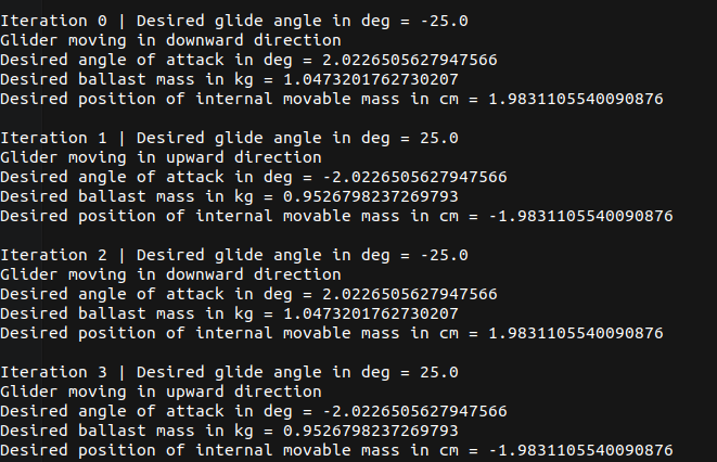
We specify the desired glide path angle to be $\xi_d = \deg{25}$ and desired glider speed as $V_d = 0.3 m/s$. These same values are used throughout to obtain plots for sawtooth as well as spiral motions.

Upon calculating the values at glide equilibrium for the downward dive at $t=0$, we get the values shown in Table 4.4.

$\xi_d$	-25 deg
$\theta_d$	-23 deg
$\alpha_d$	2 deg
$v_{1_d}$	0.299 m/s
$v_{3_d}$	0.0106 m/s
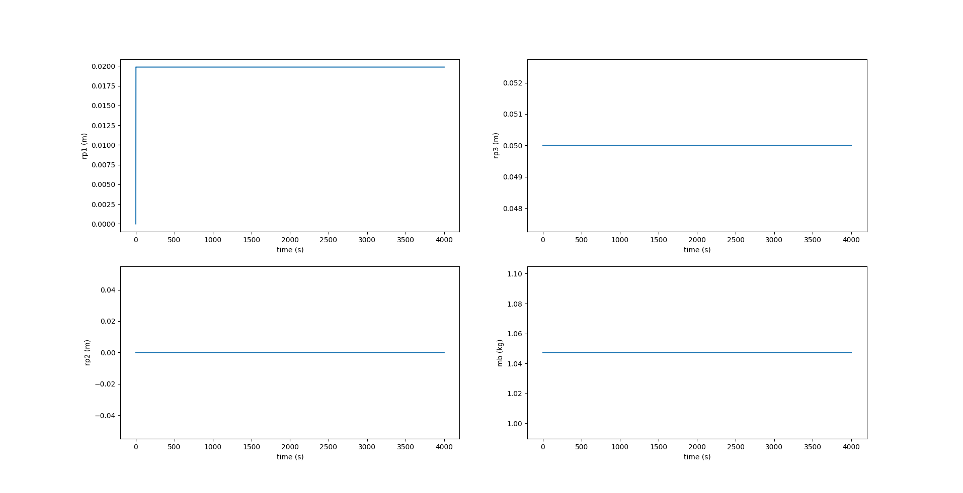
$r_{p1_d}$	0.0198 m
$r_{p3_d}$	0.05 m
$m_{b_d}$	1.047 kg

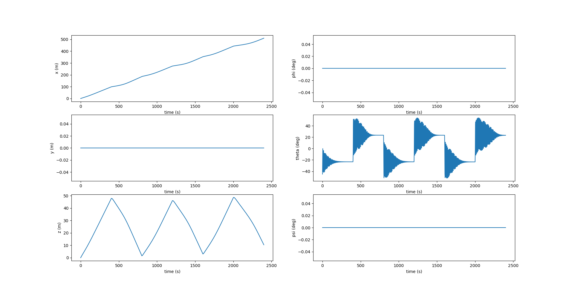
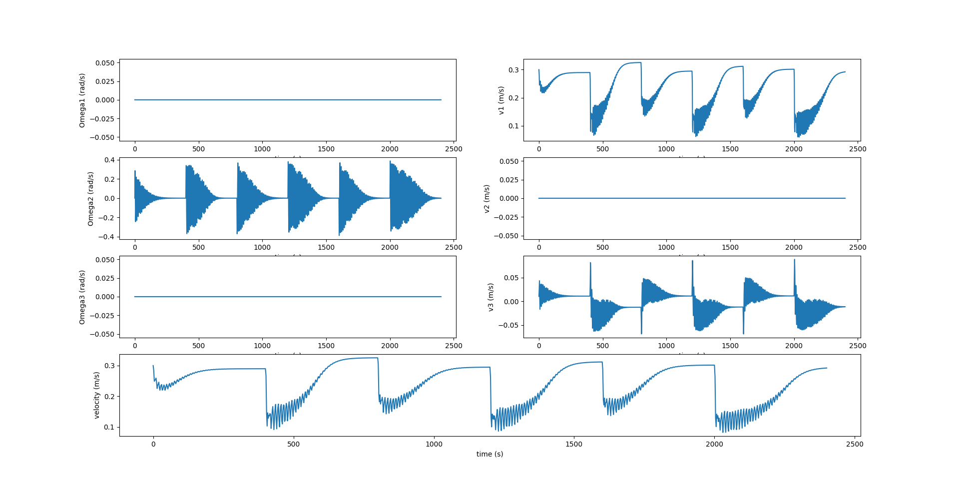
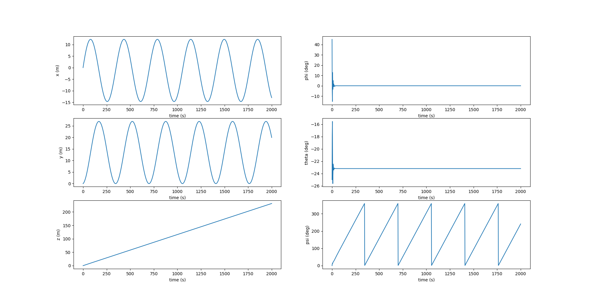
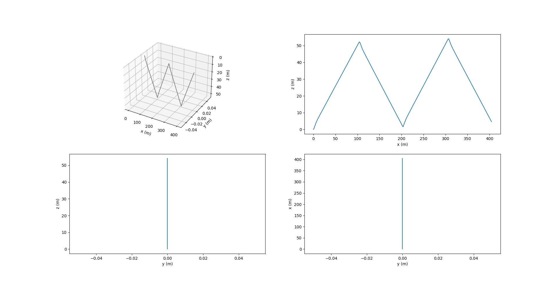
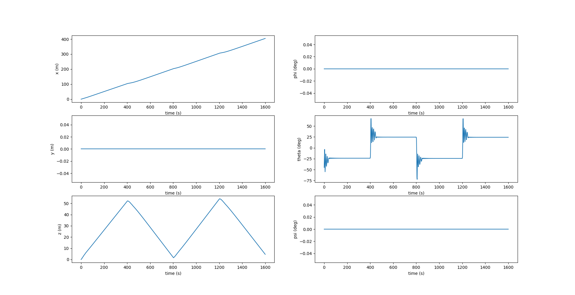
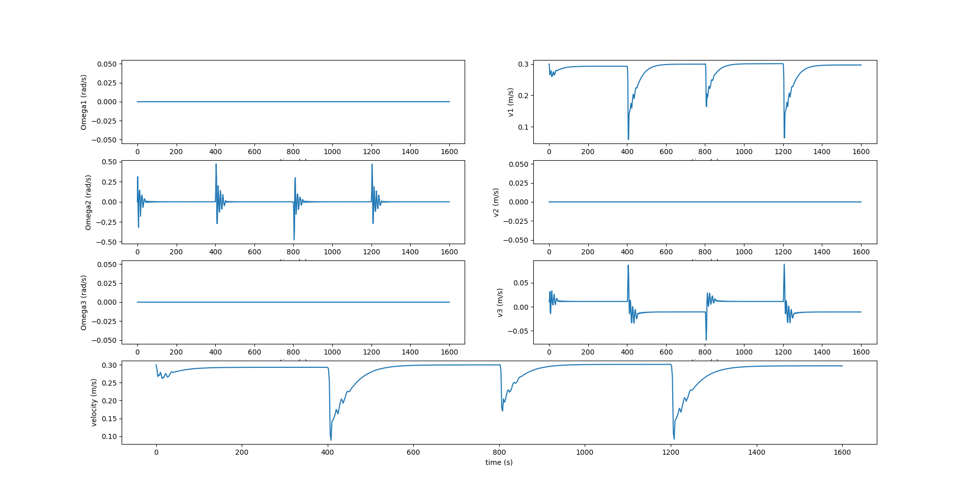
Sawtooth Motion

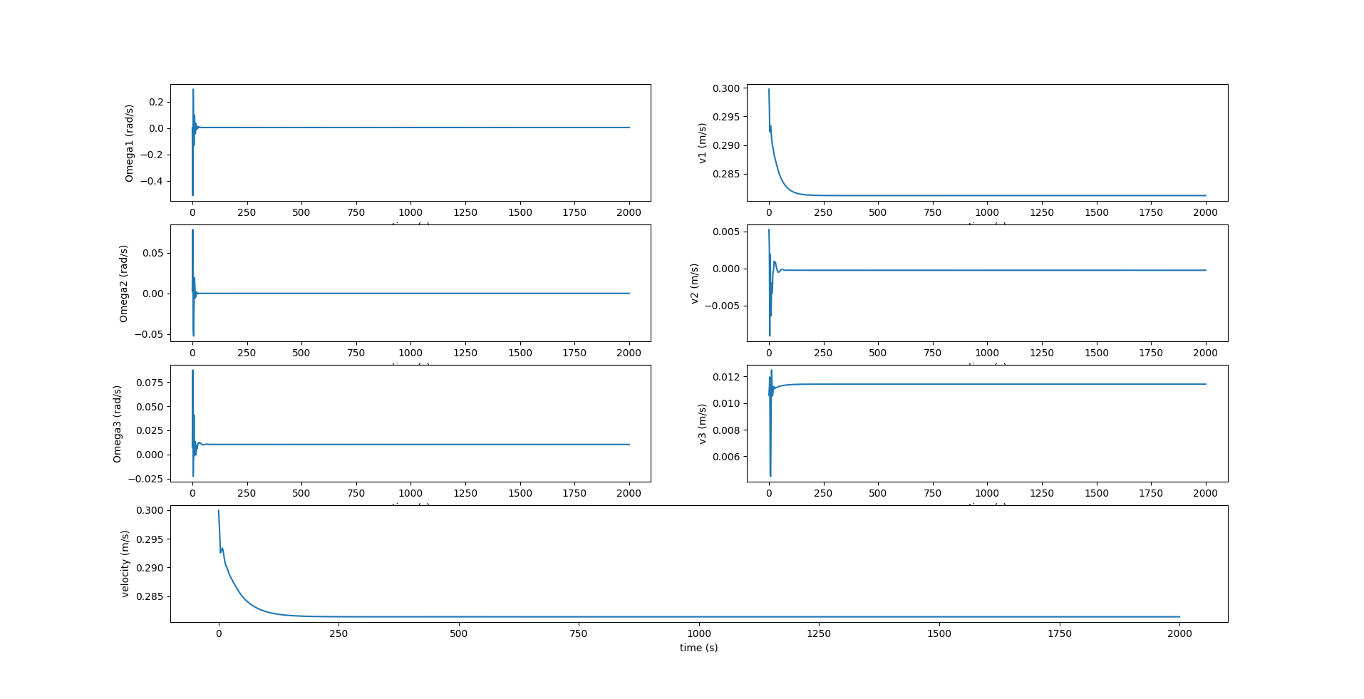
The slide-slip angle $\beta = 0$ deg since there is no component of velocity along the $Y_0$ axis, due to which the viscous side force $SF$ and moments $M_{DL_1}$, $M_{DL_3}$ are all equal to $0$.

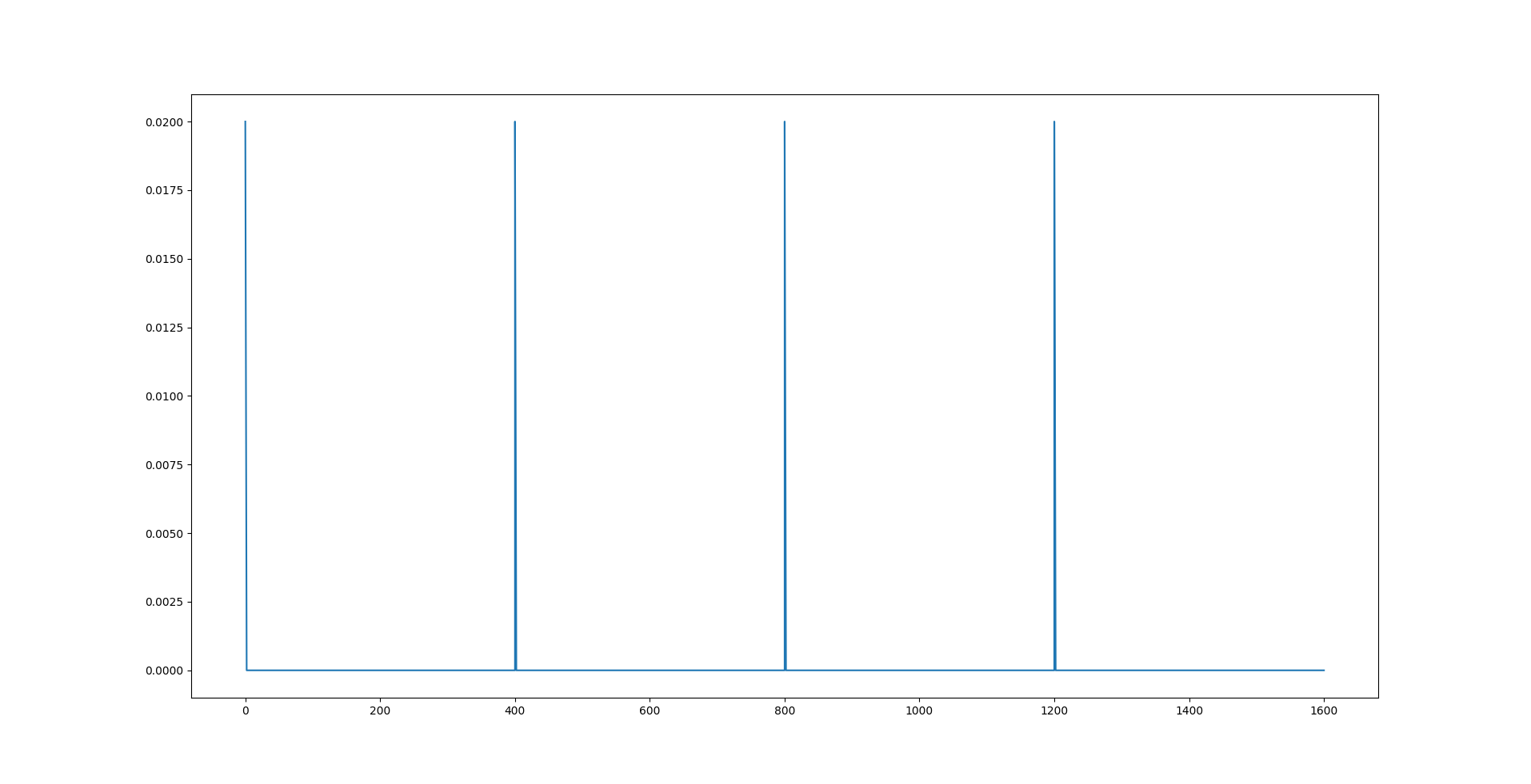
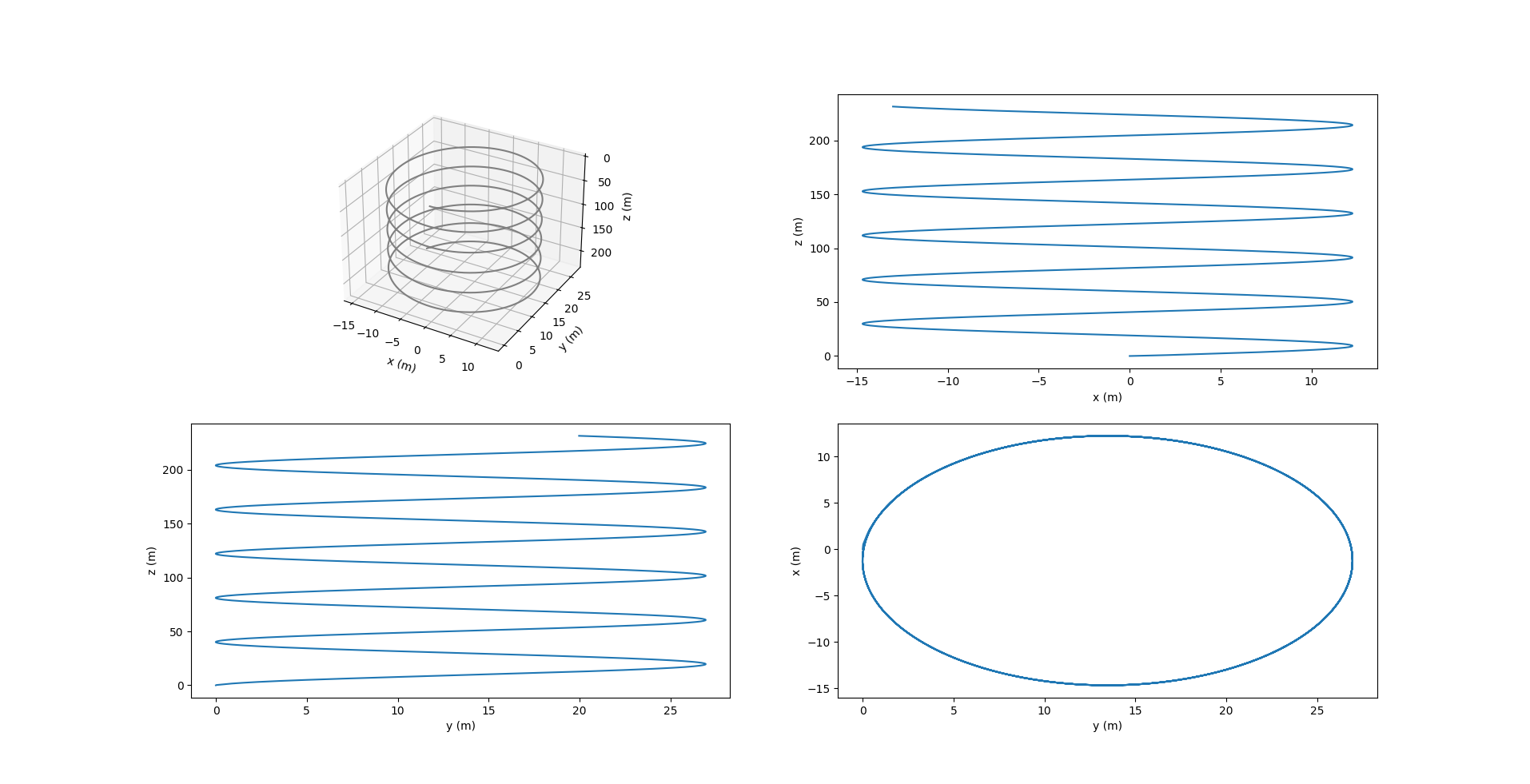
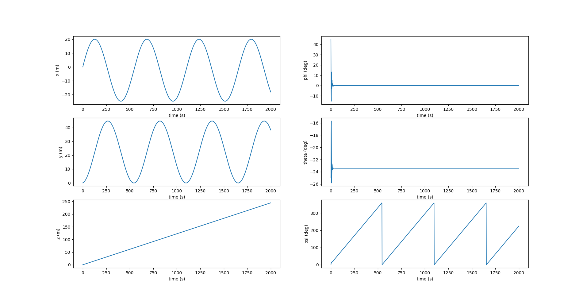
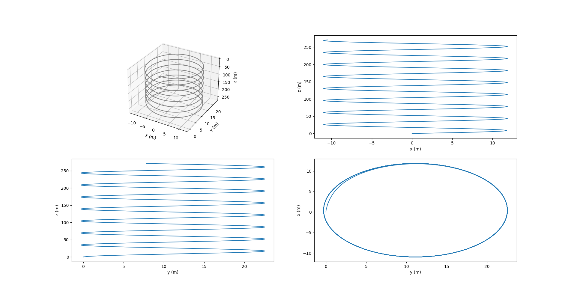
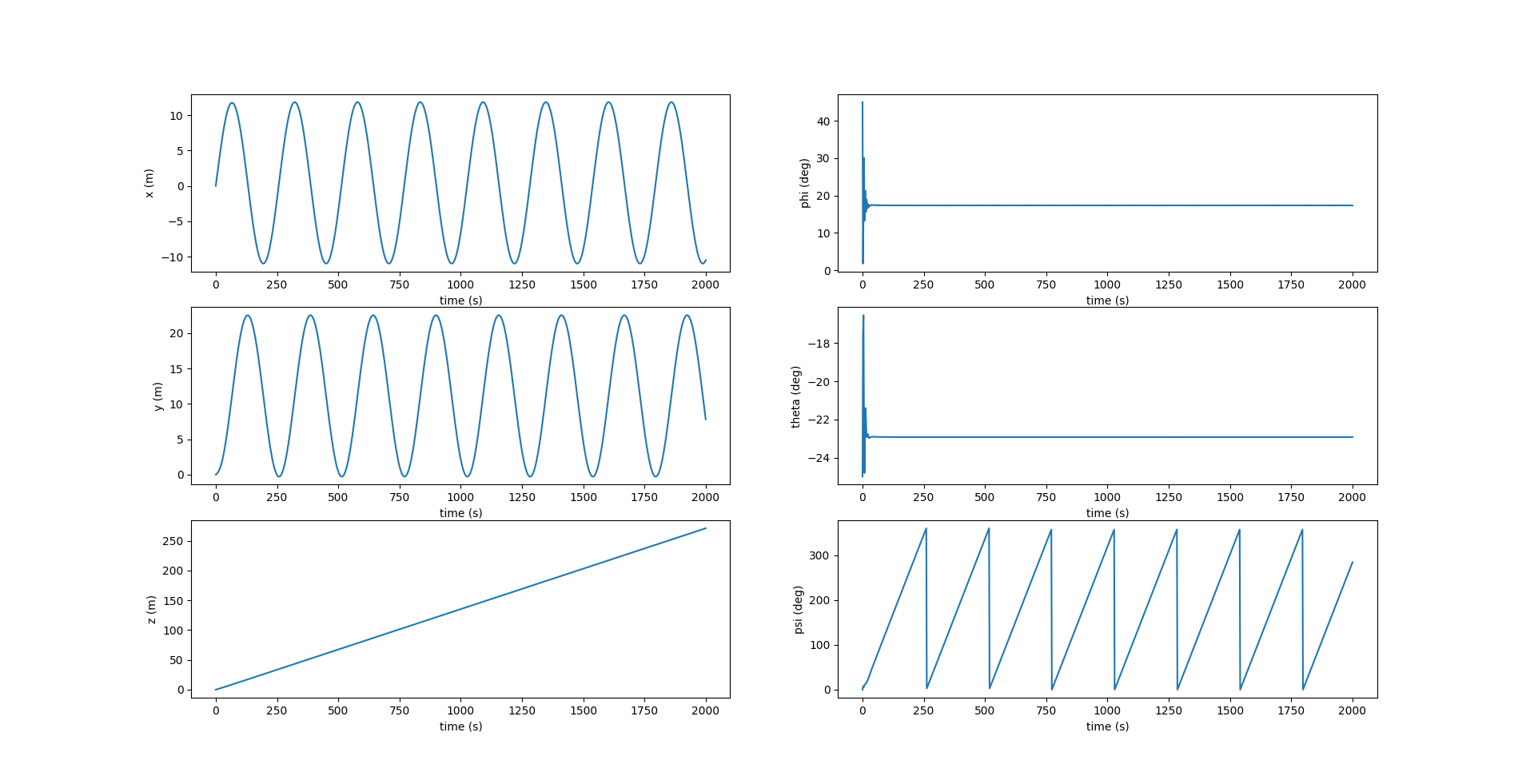
The images below show the sawtooth trajectory and the relevant plots for 4 cycles (1 cycle is considered to be 1 upward or downward motion).

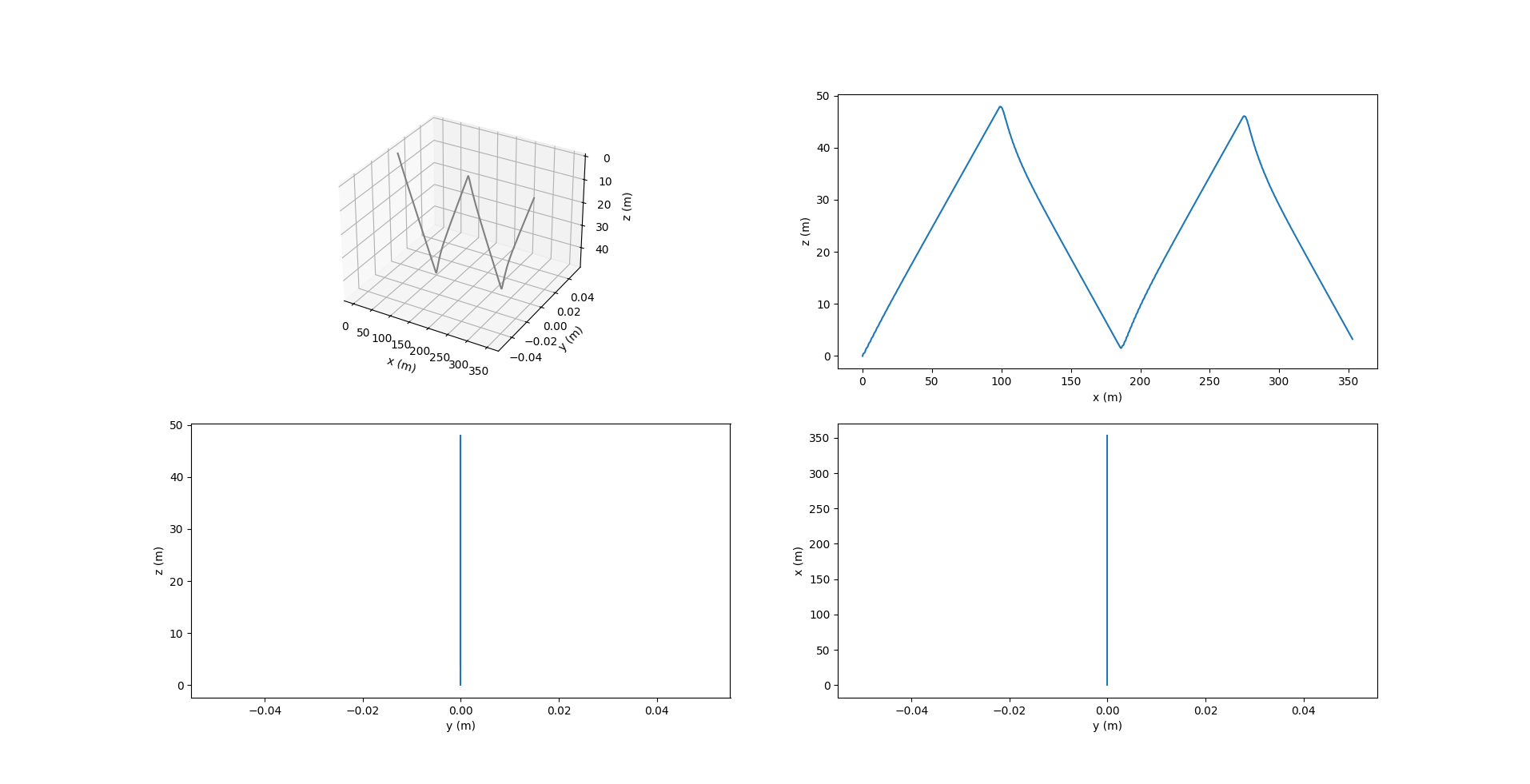
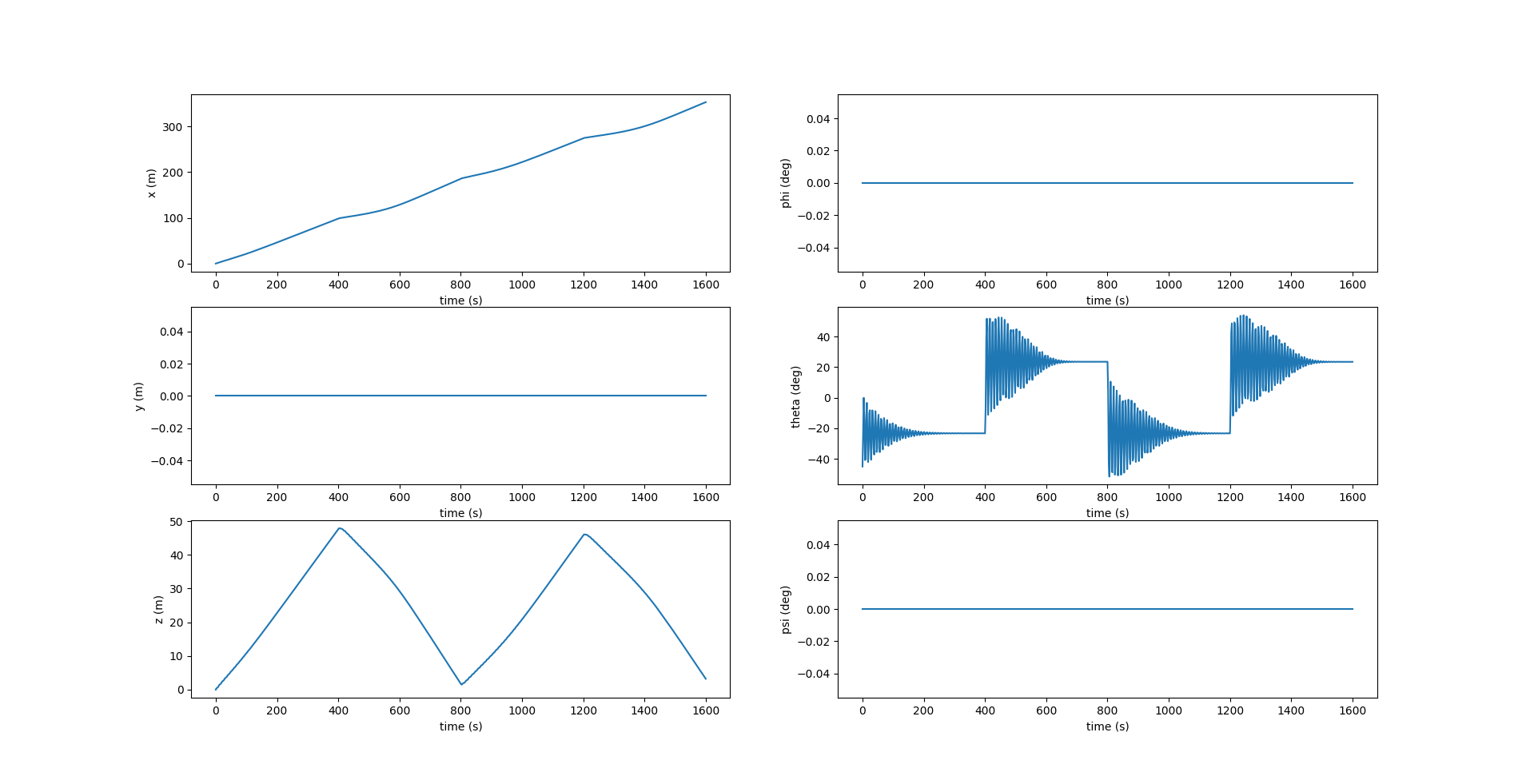
Notice in the above figure, $y$ remains zero at all times since the motion is restricted to the $xz$ plane. The roll $\phi$ and yaw $\psi$ are also zero, while the pitch $\theta$ changes at each inflection.

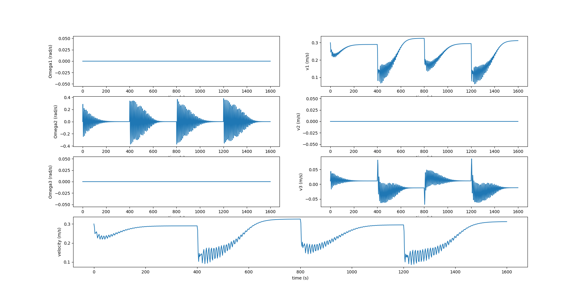
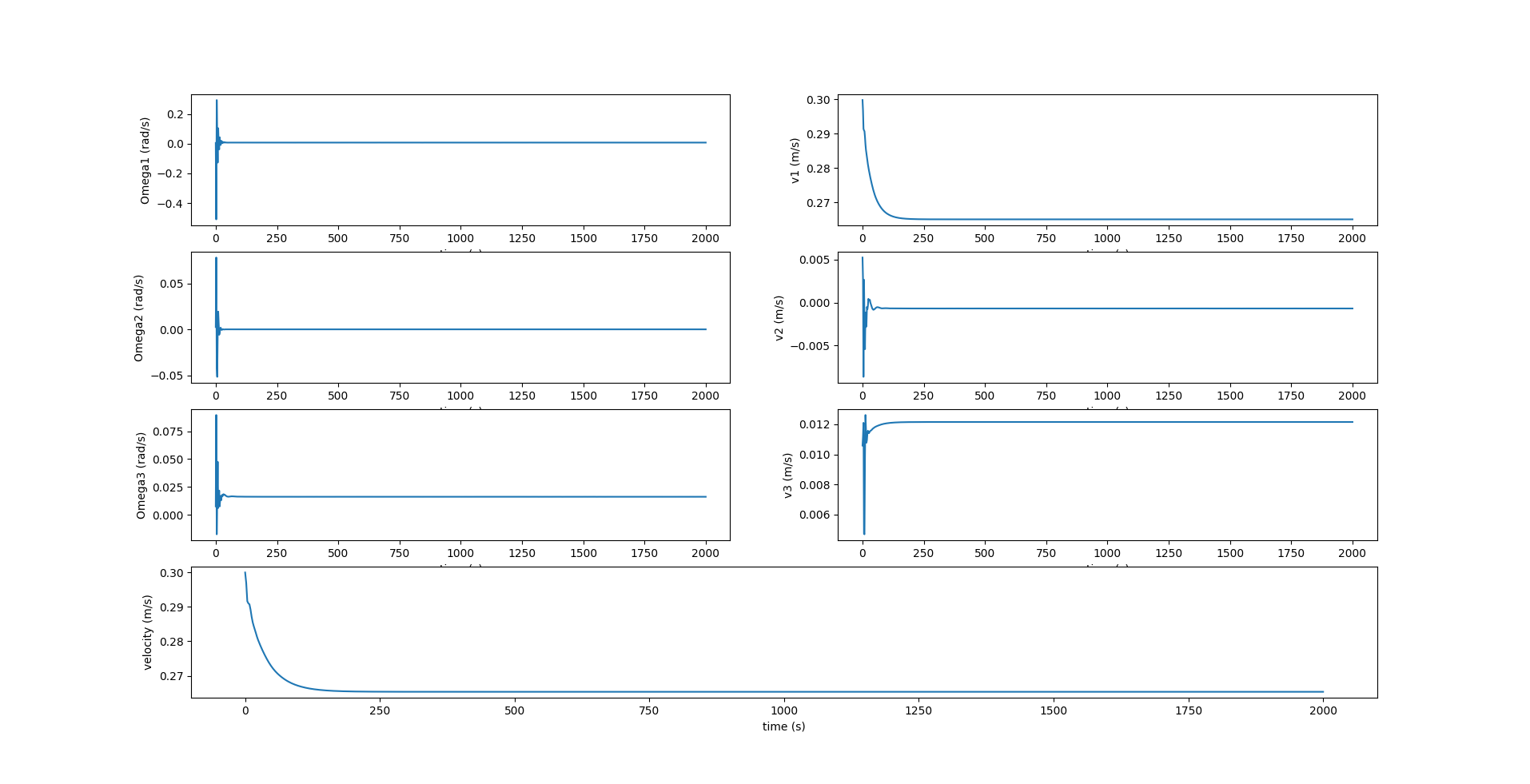
In the above figure, $\Omega_1, \Omega_3$ are zero since there is no rotation about the $X_0$ and $Z_0$ axes. $v_2$ is also zero since there is no component of velocity in the lateral direction.

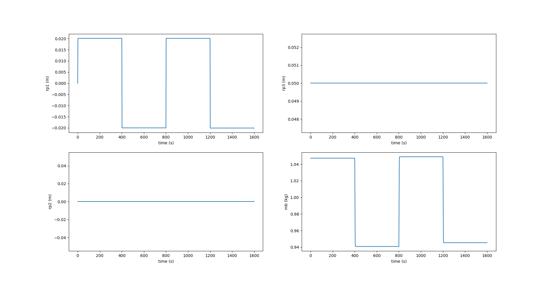
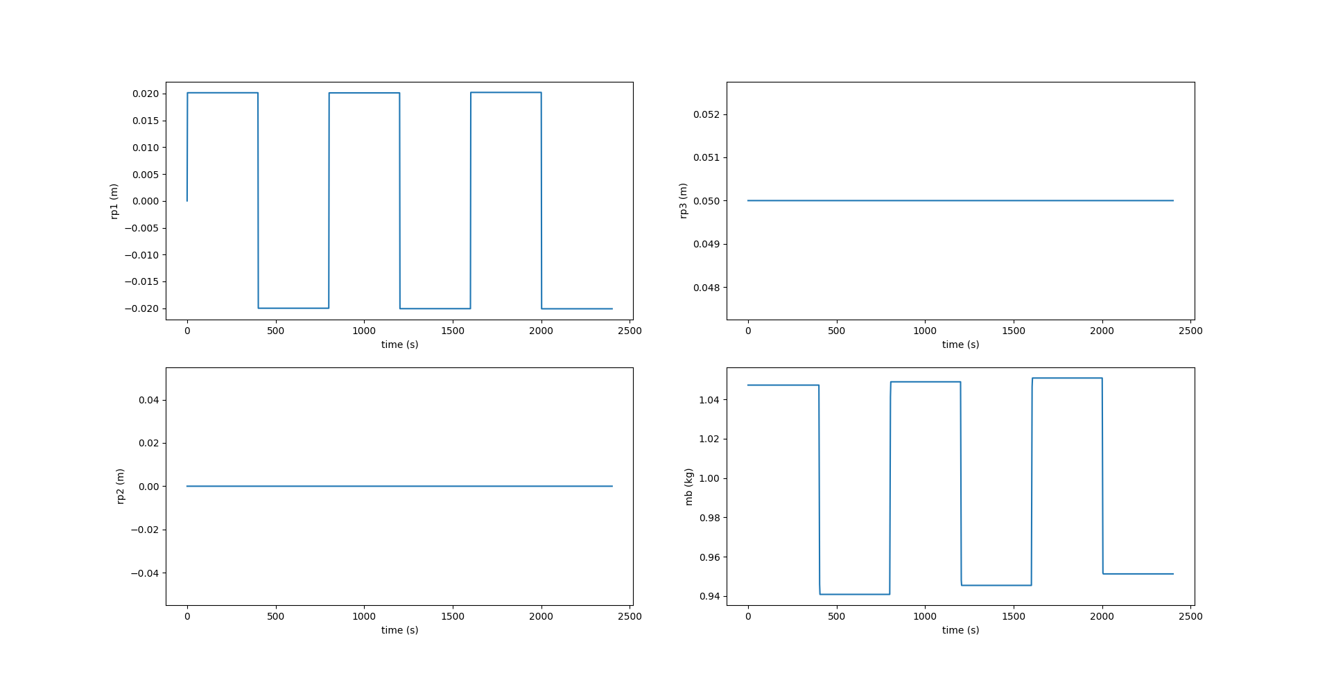
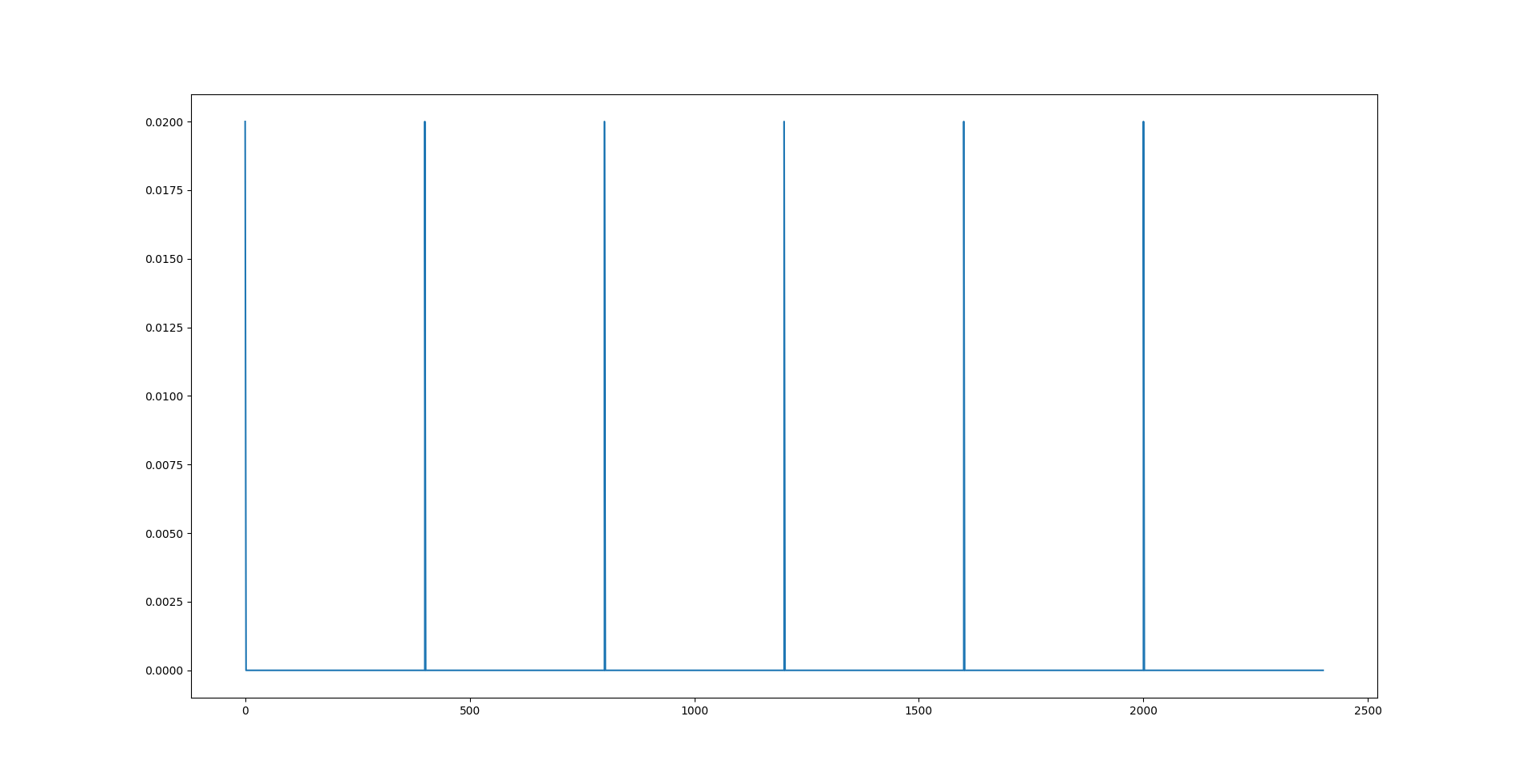
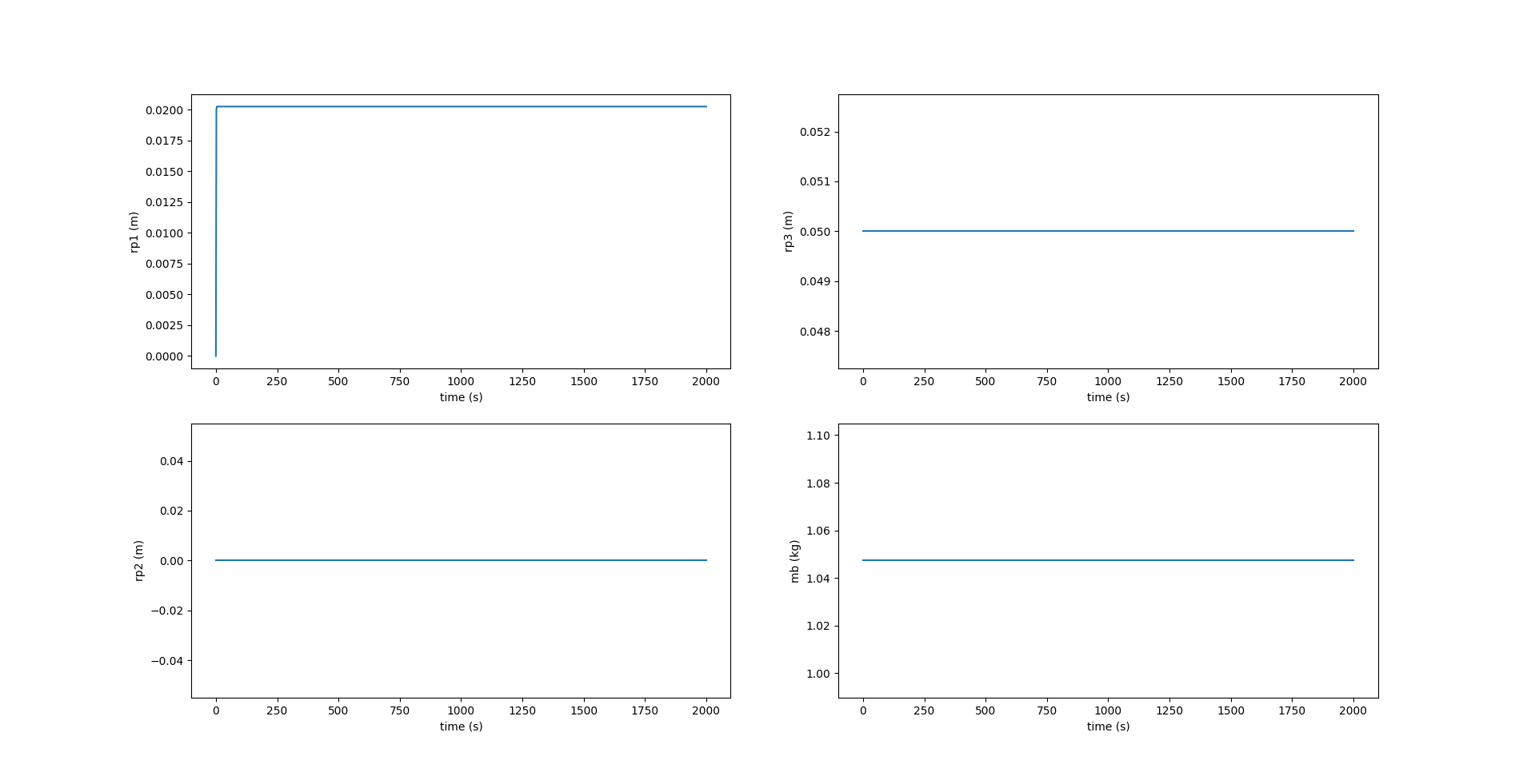
Here, we see that the component of \(\boldsymbol{r_p}\) along $X_0$ axis, i.e., $r_{p1}$ reaches the desired position \(r_{p1_d}\) at each inflection. \(r_{p2}\) is zero while \(r_{p3}\) is fixed at \(5 \space cm\). The image below shows the change in values of acceleration given to \(\bar{m}\) to change its position \(r_{p1}\) along the \(X_0\) axis. A value of \(0.02 \space m/s^2\) is given at the beginning of each inflection and remains zero at every other instant.

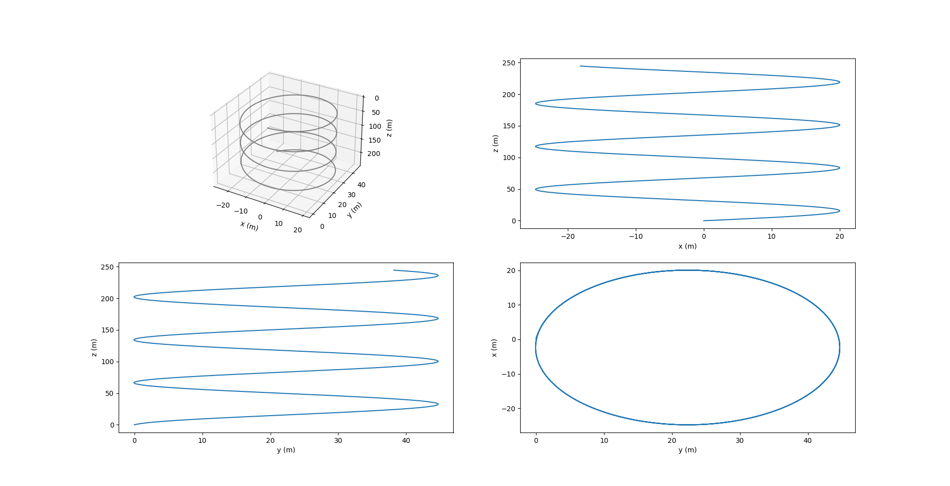
The simulator also allows us to simulate the sawtooth motions for \textit{n} number of cycles with the -c CYCLE or –cycle CYCLE argument. The images below show the sawtooth trajectory and the relevant plots for 6 cycles. The plots are similar to the ones shown above.

Spiral Motion

The presence of a side-slip angle, given by equation (3.22), results in a side force and hydrodynamic moments \(M_{DL_1}, M_{DL_3}\), which stimulates the glider’s lateral dynamics.

As mentioned previously, gliders can actuate their heading in two ways - using a rudder or by rolling, and the subsequent plots obtained from the simulator are displayed below.

Using a Rudder

The presence of a rudder changes the hydrodynamic forces and moments, particularly the drag $D$, side force $SF$ and moment \(M_{DL_3}\). The hydrodynamic rudder coefficients are set as \(K_{D_\delta} = 2.0, K_{SF_\delta} = 5.0, K_{MY_\delta} = 1.0\), and a rudder angle $\delta$ is chosen.

As a result, the viscous forces and moments equations change as follows,

\[\begin{align} D & =\left(K_{D_0}+K_D \alpha^2 + K_{D_\delta} \delta^2\right)\left(V^2\right)\\ SF & =\left(K_{\beta}\beta + K_{SF_\delta}\delta\right)\left(V^2\right) \\ M_{D L_3} & =\left(K_{M Y} \beta +K_{q 3} \Omega_3 + K_{MY_\delta}\delta\right)\left(V^2\right) \end{align}\]

When rudder is set at $\delta = 25$ deg:

Equilibrium roll angle of glider: -0.006355428997639093 deg
Equilibrium pitch angle of glider: -23.18914824153443 deg
Sideslip angle of glider: -0.14978467830958261 deg
Equilibrium glide speed: 0.26533944912351476 m/s
Radius : 14.659688296097228 m

From the above plots, we see that the roll and pitch reach stable values, while the yaw changes at a constant rate. $r_{p2}, r_{p3}$ are zero and the ballast mass remains constant throughout the glide. When the rudder is set at a high angle, it forces the glider to spiral down in a smaller circle, and hence makes more spirals in the given simulation time (2000s).

When rudder is set at a smaller angle, the glider moves along a circle of larger radius, and hence makes lesser spirals in the given time. The plots when the rudder is set at $\delta = 15$ deg are shown below:

Equilibrium roll angle of glider: -0.061902809708920835 deg
Equilibrium pitch angle of glider: -23.41541331190702 deg
Sideslip angle of glider: -0.04893320699757756 deg
Equilibrium glide speed: 0.28140084245628366 m/s
Radius : 24.39382252404712 m

Rolling to Turn

While in most AUGs, such as the Slocum glider, the internal movable mass $\bar{m}$ has only 1 DOF and uses a rudder to turn, this simulator just offers an additional functionality to move $\bar{m}$ even along the lateral $Y_0$ axis to produce a roll, and thereby induce a yaw. Here, $r_{p2_d}$ is set as 0.02 m and is the amount by which $\bar{m}$ moves along $Y_0$.

Equilibrium roll angle of glider: 17.338401948861858 deg
Equilibrium pitch angle of glider: -22.924819423213446 deg
Sideslip angle of glider: 3.2097452502678503 deg
Equilibrium glide speed: 0.3110046819320383 m/s
Radius : 13.07315069665681 m

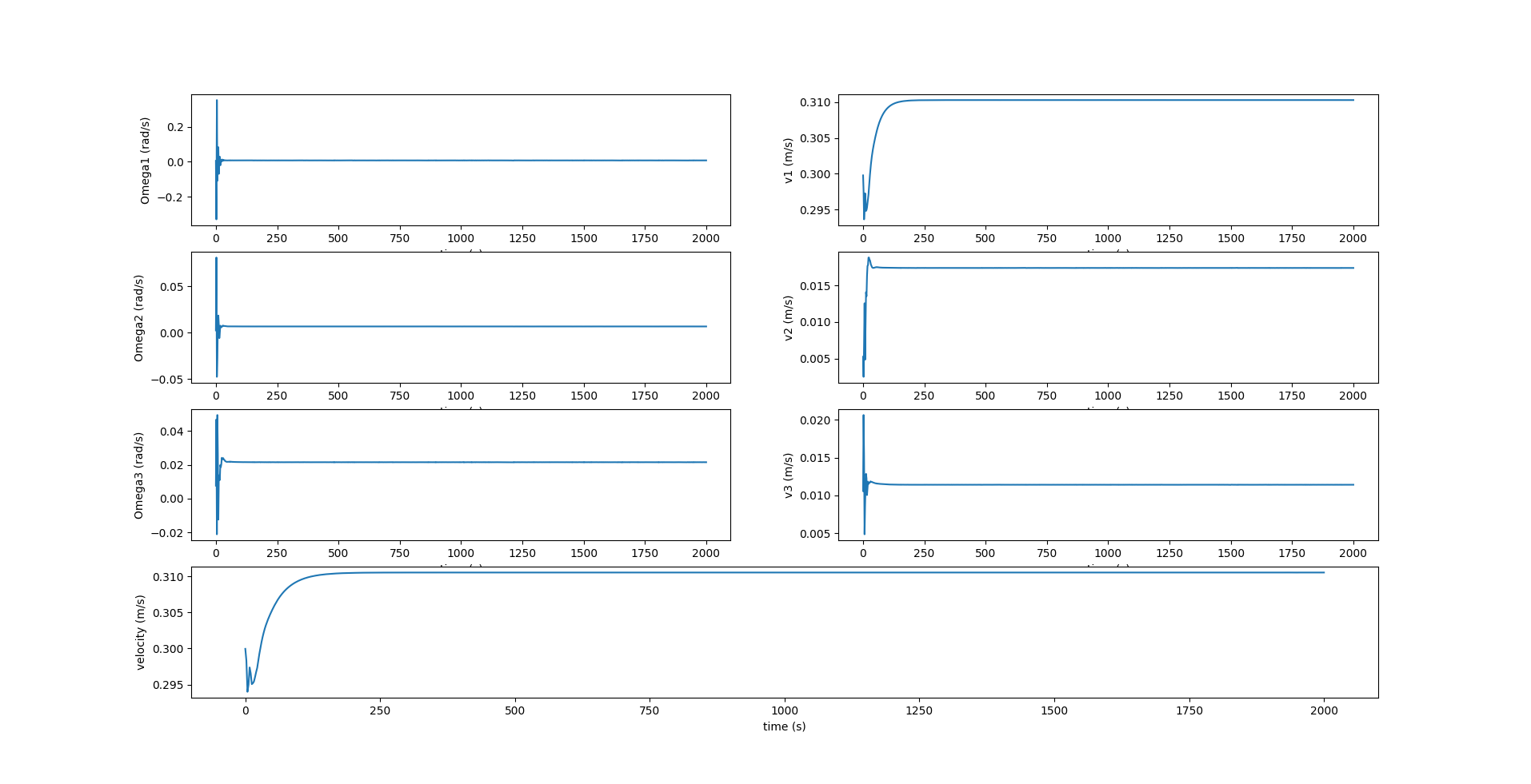
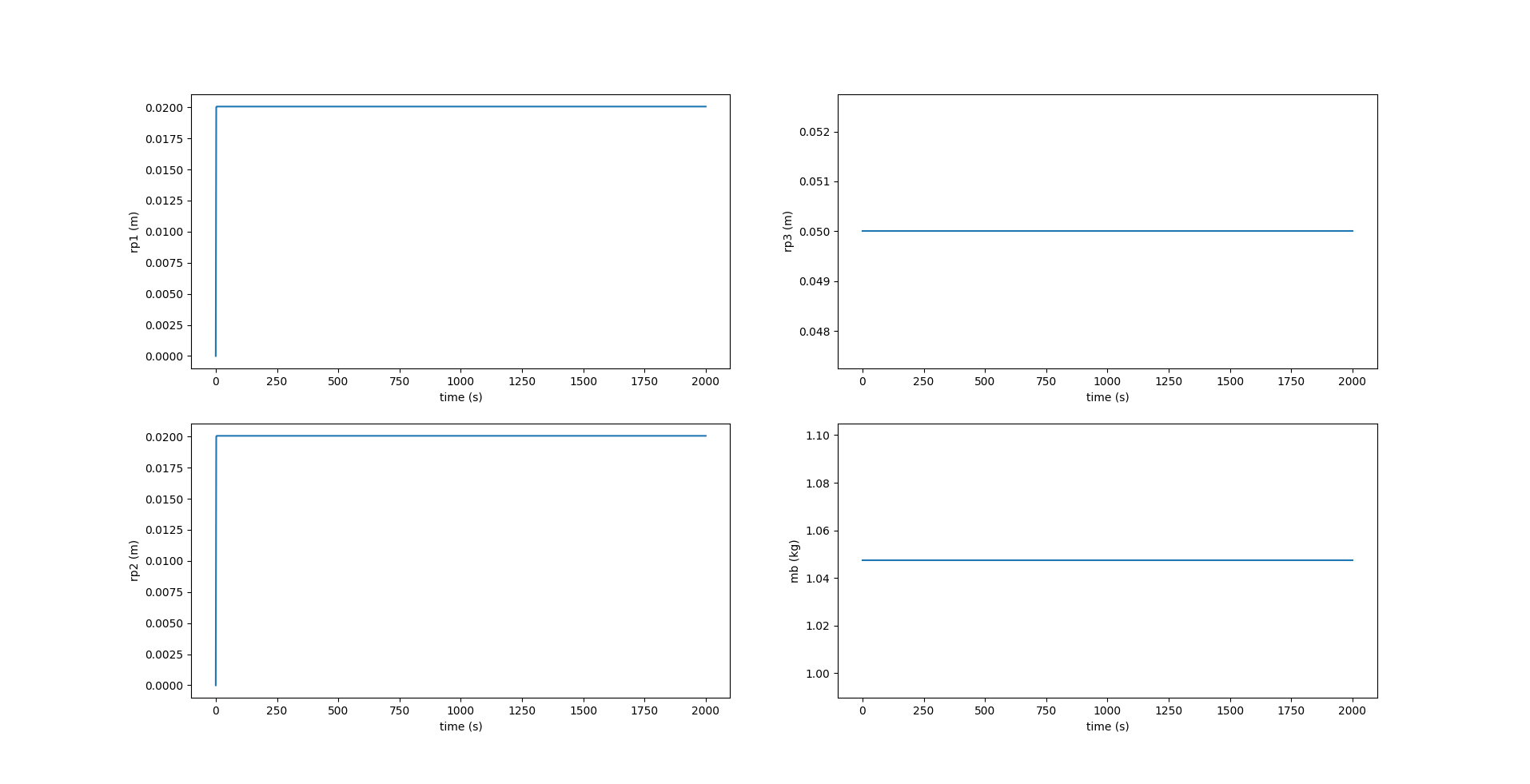
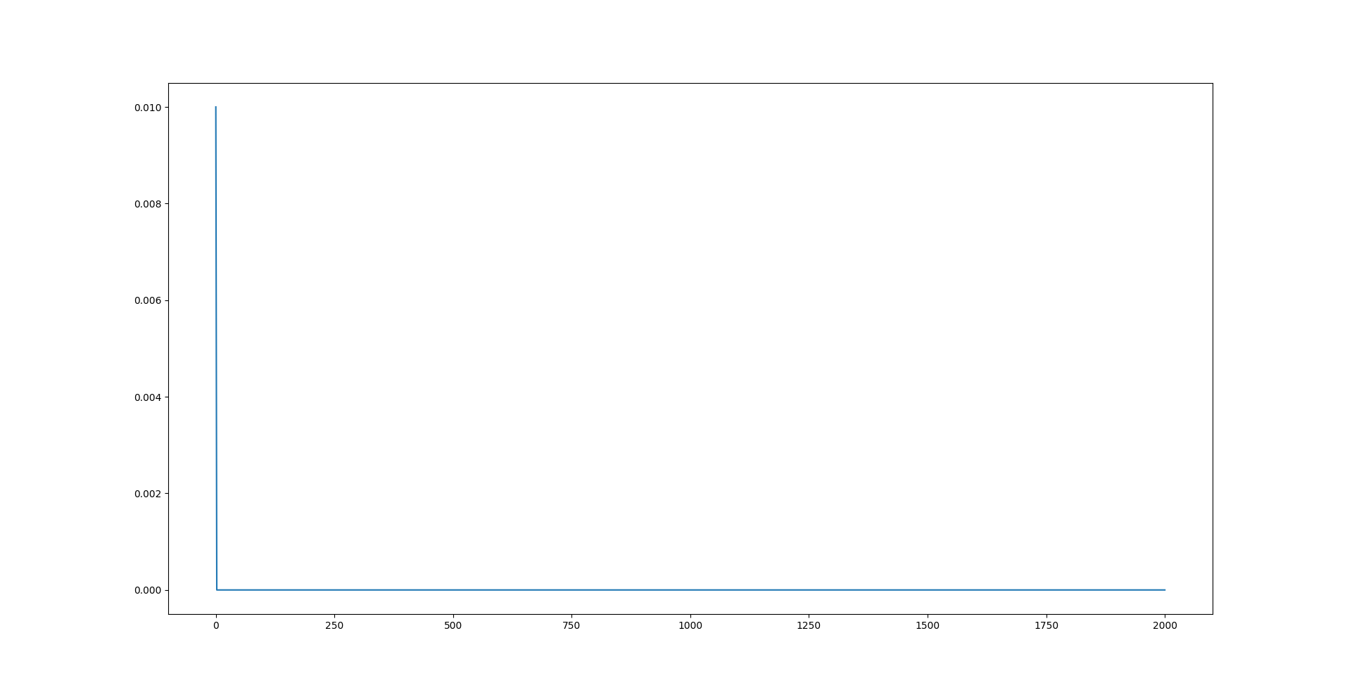
The image above shows the plots of $r_{p1}$ and $r_{p2}$ until they reach their desired values. $r_{p3}$ is fixed at \(0.05 \space m\) throughout the glide. The figure below shows the acceleration $w_{p2}$ given to $\bar{m}$ to change $r_{p2}$.

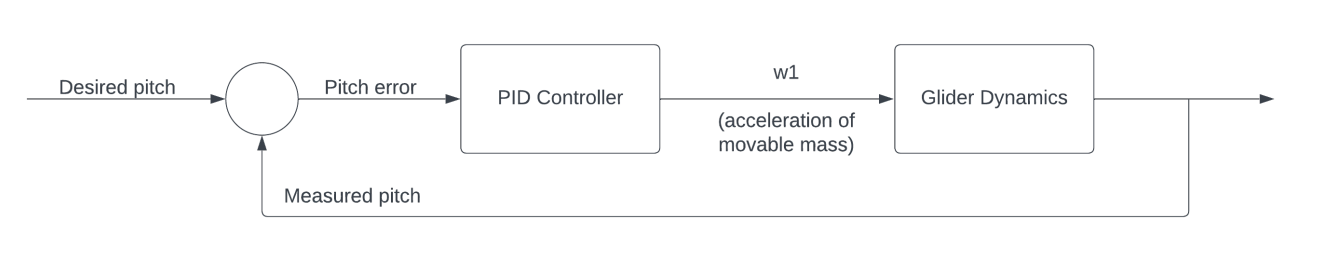
PID Control

To maximize the benefits of underwater gliders in ocean sampling and other applications, a reliable control system is crucial. Efficient gliding, whether precise elevation or heading, depends on precise control. Improvements in control enhance gliders’ utility in scientific missions, with feedback systems ensuring robustness against disturbances during prolonged missions.

In this thesis, two types of PID (Proportional Integral Derivative) controllers are presented - one for pitch control and the other for yaw control.

Sawtooth Pitch Control

Essentially a PD controller, the gain values are set as $K_p = 0.05, K_i = 0.0, K_d = 0.0005$. The controller takes in the current value of the pitch $\theta$ and the desired reference value of pitch $\theta_d$ as the inputs and outputs the acceleration of the internal movable mass $\bar{m}$ to control its position $\boldsymbol{r_p}$.

The plots below are similar to the ones presented previously in the sawtooth motion results but with much lesser fluctuations of the glider pitch $\theta$.

Since the model is again restricted to the $xz$ plane, the values of $y, \phi, \psi, \Omega_1, \Omega_3, v_2$ are always zero.

In the figure above, we see that $r_{p1}$ varies to obtain a more controlled pitch, as opposed to what we see in Figure 4.15. Figure 5.6 shows the acceleration $w_{p1}$ applied to the internal movable mass $\bar{m}$ along $X_0$ axis, which is the output of the PID controller, and causes $r_{p1}$ to change.

Heading Control with Rudder

A PD controller, the gain values are set as $K_p = 0.05, K_i = 0.0, K_d = 0.05$. The controller takes in current value of the yaw $\psi$ and the desired reference value of yaw $\psi_d$ as the inputs and outputs the desired rudder angle $\delta$, which in turn, changes the yaw of the glider.

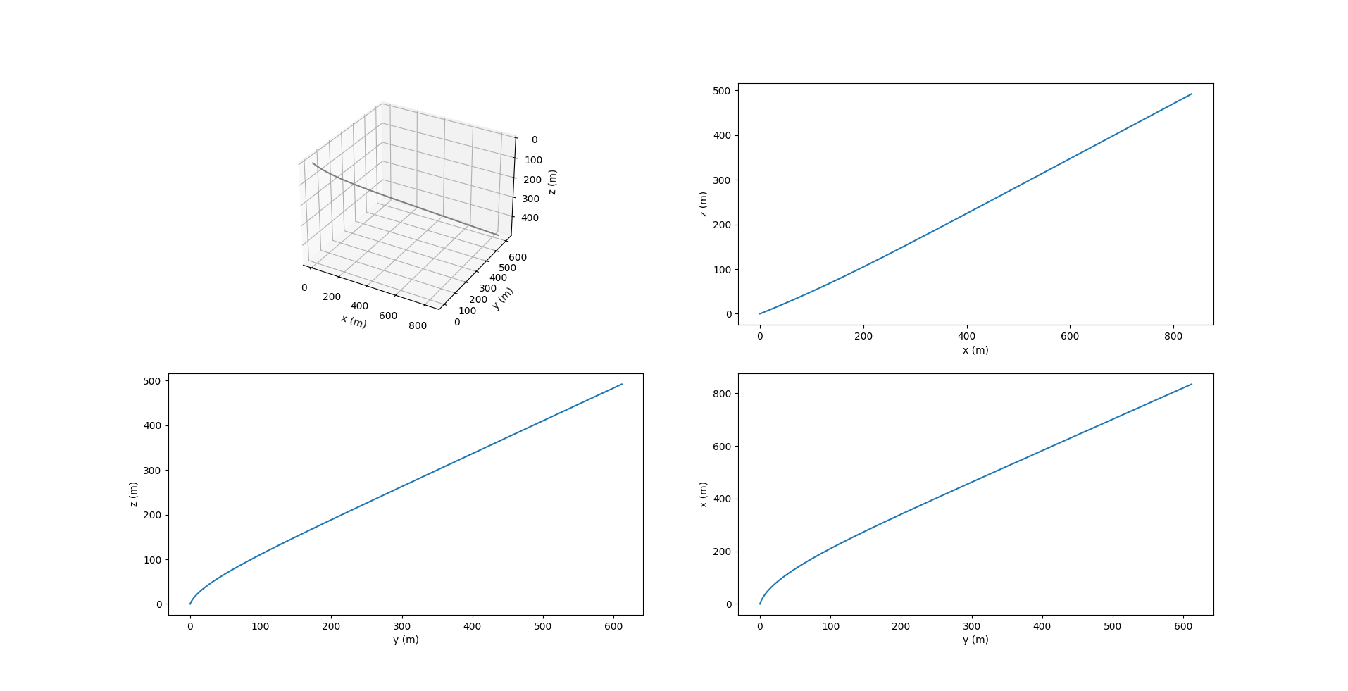
In this example, the desired yaw to be achieved $\psi_d$ is set as 40 deg, and the glide angle is the same as before. In the figure below, the blue line makes an angle of 40 deg with the x-axis and marks the desired direction of motion of the AUG. The red line shows the actual trajectory of the glider, which is fitted with the yaw controller.

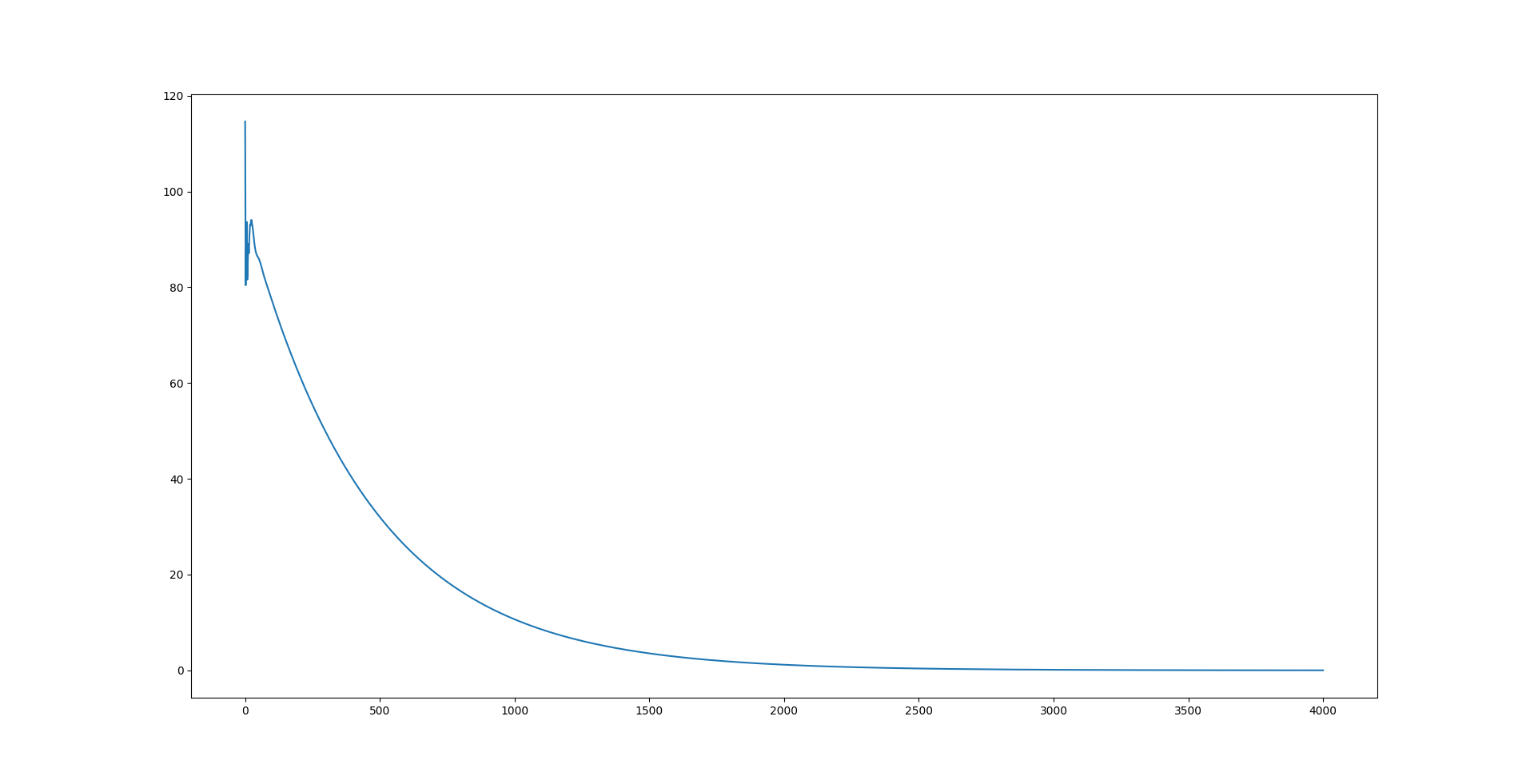
The image above shows the variation in the rudder angle, which is the output of the PID controller. Initially starting off at a high value, it varies until the yaw $\psi$ matches with the desired value $\psi_d$ and then stabilizes at zero, which means there is no further change in the yaw angle.

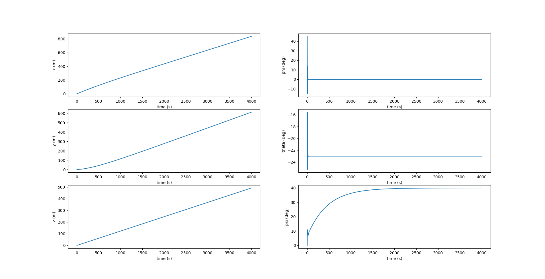
The image above shows the variation of the yaw as it starts at 0 deg and reaches the desired value $\psi_d = 40$ deg.

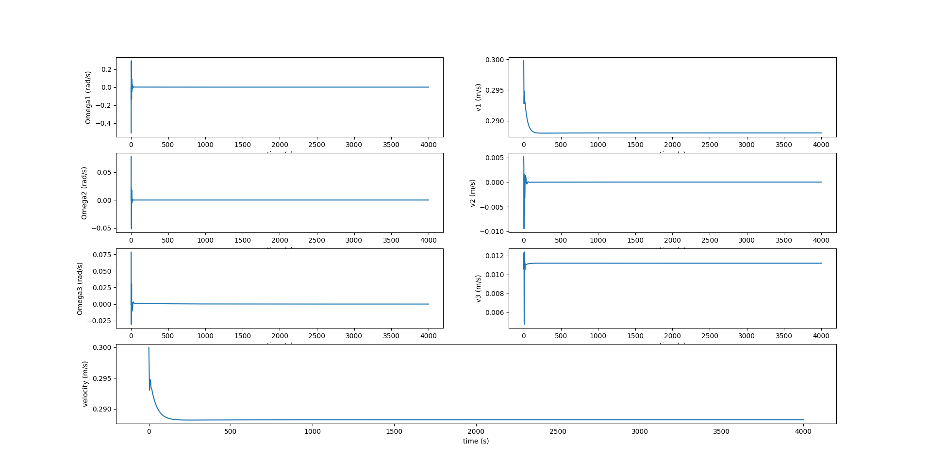
The image below shows the variation of $r_{p1}$ to reach the desired pitch $\theta_d$, as done previously.