
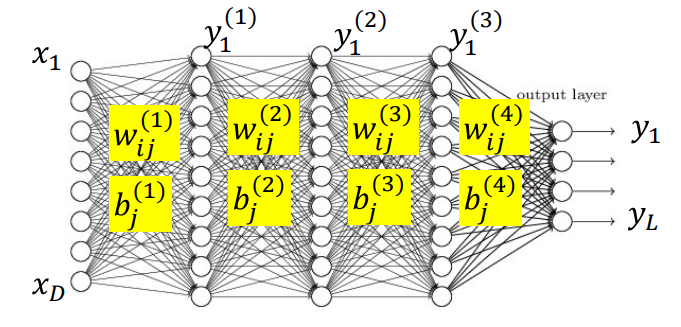
Neural Networks
Depth - length of longest path from source to sink Layer - Set of all neurons which are all at the same depth with respect to the source
Gradient
For a scalar function $f(x)$ with a multivariate input $x$:
\[df\left( x\right) =\nabla _{x}f\left( x\right) dx\] \[\nabla _{x}f\left( x\right) =\left[ \dfrac{\partial f}{\partial x_{1}}\dfrac{\partial f}{\partial x_{2}}\ldots \dfrac{\partial f}{\partial x_{n}}\right]\]Because it is a dot product, for an increment $dX$ of any given length, $df$ is maximum if the increment $dX$ is aligned with the gradient direction $\nabla _{x}f\left( x\right)^T$. So the gradient is the direction of steepest ascent.
So if you want a function to decrease, your increment should be in the direction of $-\nabla _{x}f\left( x\right)^T$.
To find a maximum move in the direction of gradient:
\[x^{k+1} = x^k + \eta^k \nabla_x f(x^k)^T \\[1em]\]To find a minimum move in the direction of gradient:
\[x^{k+1} = x^k - \eta^k \nabla_x f(x^k)^T \\[1em]\]There are many solutions to choosing step size $\eta^k$.
Hessian
\[\nabla^2_{x} f(x_1, \ldots, x_n) = \begin{bmatrix}\frac{\partial^2 f}{\partial x_1^2} & \frac{\partial^2 f}{\partial x_1 \partial x_2} & \cdots & \frac{\partial^2 f}{\partial x_1 \partial x_n} \\\frac{\partial^2 f}{\partial x_2 \partial x_1} & \frac{\partial^2 f}{\partial x_2^2} & \cdots & \frac{\partial^2 f}{\partial x_2 \partial x_n} \\\vdots & \vdots & \ddots & \vdots \\\frac{\partial^2 f}{\partial x_n \partial x_1} & \frac{\partial^2 f}{\partial x_n \partial x_2} & \cdots & \frac{\partial^2 f}{\partial x_n^2}\end{bmatrix}\]Network
A continuous activation function applied to an affine function of the inputs
\[y = f\left( \sum_i w_i x_i + b \right) \\[1em] y = f(x_1, x_2, \ldots, x_N; W)\]Activation Functions and Derivatives
Sigmoid:
\[f(z) = \frac{1}{1 + \exp(-z)} \\f'(z) = f(z)(1 - f(z)) \\[1.5em]\]Tanh:
\[f(z) = \tanh(z) \\f'(z) = 1 - f^2(z)\]ReLU:
\[f(z) = \begin{cases}z, & z \geq 0 \\0, & z < 0\end{cases} \\f'(z) = \begin{cases}1, & z \geq 0 \\0, & z < 0\end{cases} \]Softplus:
\[f(z) = \log(1 + \exp(z)) \\f'(z) = \frac{1}{1 + \exp(-z)}\]Softmax:
\[f(z_i) = \frac{e^{z_i}}{\sum_{j=1}^{K} e^{z_j}} \\ f'(z_i) = \begin{cases} f(z_i)(1 - f(z_i)), & \text{if } i = j \\ - f(z_i) f(z_j), & \text{if } i \ne j \end{cases}\]Training by Back Propagation
Forward Pass
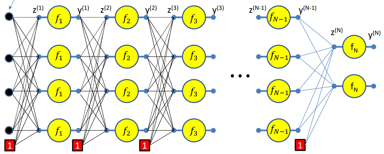
Setting $y_i^{(0)} = x_i$ and $w_{0j}^{(k)} = b_j^{(k)}$. Let the bias equal $1$ for simplicity.
For layer 1,
\[z_j^{(1)} = \sum_i w_{ij}^{(1)}y_i^{(0)} \\ y_j^{(1)} = f_1(z_j^{(1)})\]For layer 2,
\[z_j^{(2)} = \sum_i w_{ij}^{(2)}y_i^{(1)} \\ y_j^{(2)} = f_2(z_j^{(2)})\]Similarly,
\[z_j^{(N)} = \sum_i w_{ij}^{(N)}y_i^{(N-1)} \\ y_j^{(N)} = f_N(z_j^{(N)})\]Backward Pass
Step 1: Initialize Gradient at Output Layer
We start by computing the gradient of the loss w.r.t. the network output:
\[\frac{\partial Div}{\partial y^{(N)}_i} = \frac{\partial Div(Y, d)}{\partial y_i}\]Then, propagate this to the pre-activation output $z^{(N)}$:
\[\frac{\partial Div}{\partial z^{(N)}_i} = \frac{\partial y_i^{(N)}}{\partial z_i^{(N)}} \cdot \frac{\partial Div}{\partial y^{(N)}_i} =f_N'\left(z^{(N)}_i\right) \cdot \frac{\partial Div}{\partial y^{(N)}_i}\]In case of a vector activation function, such as the softmax function, $y_i^{(N)}$ is influenced by every $z_i^{(N)}$:
\[\frac{\partial Div}{\partial z_i^{(N)}} = \sum_j \frac{\partial y_j^{(N)}}{\partial z_i^{(N)}} \cdot \frac{\partial Div}{\partial y_j^{(N)}}\]Step 2: Backpropagation Through Layers
Loop from layers $k = (N-1) \rightarrow 0$:
For each layer $k$ and for each neuron $i$ in that layer:
Compute gradient of loss w.r.t. activation:
\[\frac{\partial Div}{\partial y^{(k)}_i} = \sum_j w_{ij}^{(k+1)} \cdot \frac{\partial Div}{\partial z^{(k+1)}_j}\]Chain through activation function:
\[\frac{\partial Div}{\partial z^{(k)}_i} = \frac{\partial y_i^{(k)}}{\partial z_i^{(k)}} \cdot \frac{\partial Div}{\partial y^{(k)}_i} = f_k'\left(z^{(k)}_i\right) \cdot \frac{\partial Div}{\partial y^{(k)}_i}\]Step 3: Gradient w.r.t. Weights
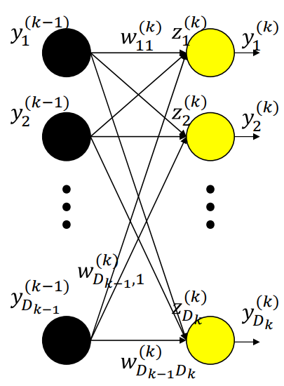
For each weight connecting neuron $i$ in layer $k$ to neuron $j$ in layer $k$:
\[\frac{\partial Div}{\partial w_{ij}^{(k)}} = y^{(k-1)}_i \cdot \frac{\partial Div}{\partial z^{(k)}_j}\]Step 4: Updating Weights
Actual loss is the sum of the divergence over all training instances:
\[Loss = \frac{1}{|\{X\}|}\sum_X Div(Y(X), d(X))\]Actual gradient is the average of the derivatives computed for each training instance:
\[\nabla_W Loss = \frac{1}{|\{X\}|}\sum_X \nabla_W Div(Y(X), d(X))\] \[W \leftarrow W - \eta \nabla_W Loss^T\]Summary
Vector Formulation
Setup:
- Let $\mathbf{y_n = Y}$, the network output
- Let $\mathbf{y_0 = X}$, the input
- Initialize:
- For each layer $k = N \rightarrow 1$:
- Compute the Jacobian of activation:
- This is a matrix of partial derivatives:
- Backward recursion step:
Gradient Computation for all $k$:
\[\nabla_{\mathbf{W}_k} Div = \mathbf{y}_{k-1} \cdot \nabla_{\mathbf{z}_k} Div\] \[\nabla_{\mathbf{b}_k} Div = \nabla_{\mathbf{z}_k} Div\]
Summary
1
2
3
4
5
6
7
8
9
10
11
12
13
14
15
16
17
18
19
20
21
22
23
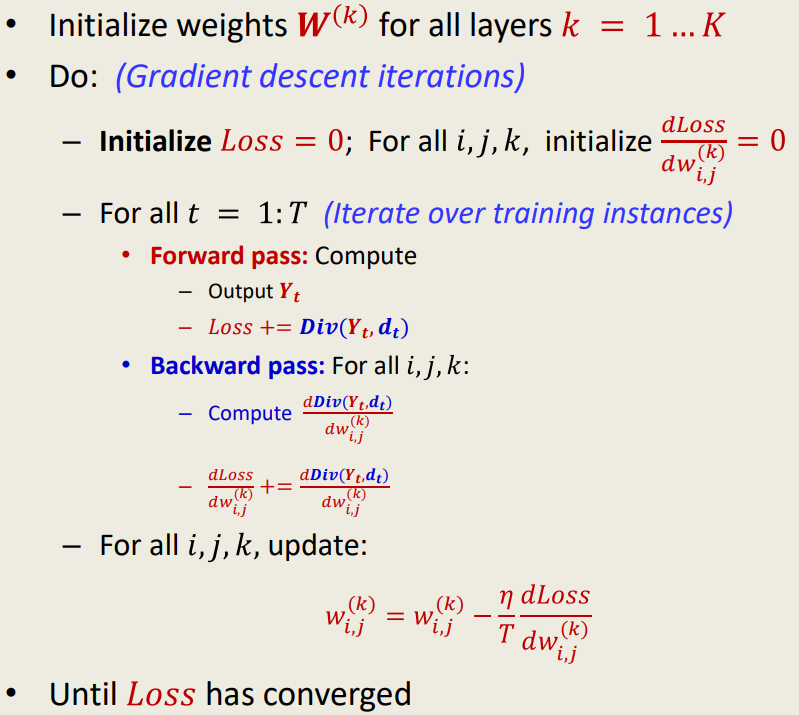
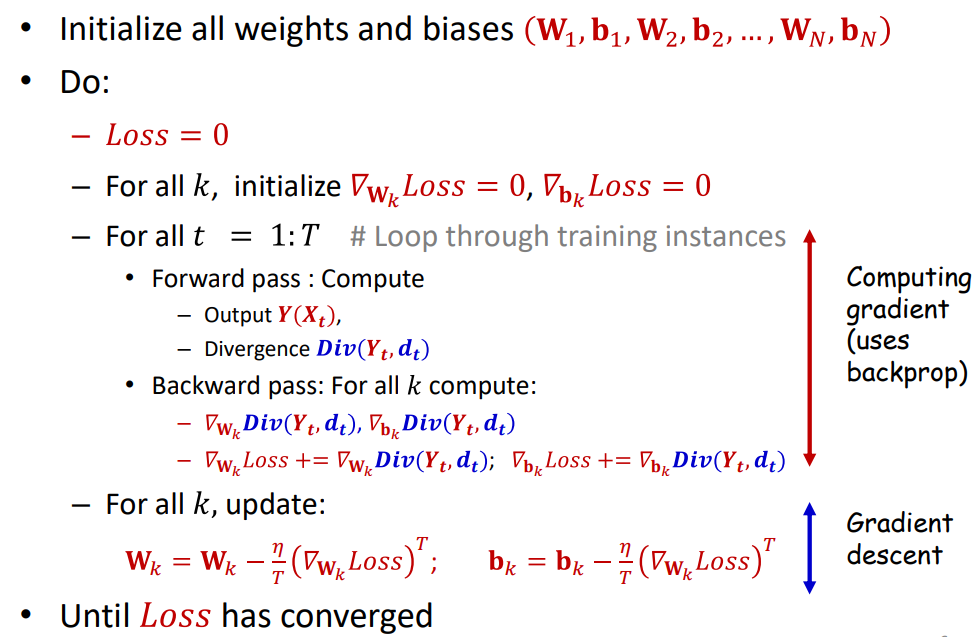
Algorithm: Batch Gradient Descent with Backpropagation
Initialize all weights and biases: W1, b1, W2, b2, ..., WN, bN
Loss ← 0
For all k:
∇Wk Loss ← 0
∇bk Loss ← 0
For t = 1 to T: # Loop through training examples
Compute output Y(Xt)
Compute divergence Div(Yt, dt)
For all k: # Backward pass
∇Wk Div(Yt, dt), ∇bk Div(Yt, dt)
∇Wk Loss ← ∇Wk Loss + ∇Wk Div(Yt, dt)
∇bk Loss ← ∇bk Loss + ∇bk Div(Yt, dt)
For all k: # Gradient Descent Update
Wk ← Wk - (η / T) * (∇Wk Loss)^T
bk ← bk - (η / T) * (∇bk Loss)^T
Repeat until Loss has converged
Important Points
- Backpropagation will often not find a separating solution even though the solution is within the class of functions learnable by the network, because the separable solution is not a feasible optimum for the loss function.
- It is minimally changed by new training instances — doesn’t swing wildly in response to small changes to the input
- It prefers consistency over perfection, due to which it works better even if there are outliers
- It is a low-variance estimator, at the potential cost of bias
- Minimizing the differentiable loss function does not imply minimizing the classification error.
Convergence of Gradient Descent
Covergence Rate
It measures how quickly an iterative optimization algorithm approaches the solution.
\[R = \left| \frac{f(x^{(k+1)}) - f(x^*)}{f(x^{(k)}) - f(x^*)} \right|\]Where:
- $x^{(k)}$: point at iteration $k$
- $x^*$: optimal point (solution)
- $f(x)$: objective function
If $R<1$, that means that the function value is getting closer to the optimum and is hence converging. The smaller the $R$, the faster the convergence.
If $R$ is a constant or upper-bounded, then the algorithm has linear convergence. This means that the difference between the function value and the optimum shrinks exponentially with iterations.
\[|f(x^{(k)}) - f(x^*)| \leq R^k \cdot |f(x^{(0)}) - f(x^*)|\]Convergence for Quadratic Surfaces
What is the optimal step size $\eta$ to reach the minimum value of the error fastest?
- Consider a general quadratic function:
- Gradient descent update:
- Taylor expansion of $E(w)$ around $w^{(k)}$:
- Newton’s method gives:
- Optimal learning rate:
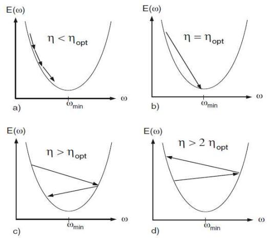
Effect of step size $\eta$:
- $\eta < \eta_{opt} \rightarrow$ monotonic convergence
- $\eta = \eta_{opt} \rightarrow$ fast convergence in one step
- $\eta_{opt}<\eta < 2\eta_{opt} \rightarrow$ oscillating convergence
- $\eta \geq 2\eta_{opt} \rightarrow$ divergence
Convergence for Multivariate Quadratic Functions
- General form of a quadratic convex function:
- If $A$ is diagonal:
This means the cost function is a sum of independent univariate quadratics. Each direction $w_i$ is uncoupled.
Equal-Value Contours:
- For diagonal $A$, the contours are ellipses aligned with coordinate axes.
- Each coordinate’s behavior is independent of the others.
Optimal Step Size:
For each dimension $i$:
\[\eta_{i,\text{opt}} = \frac{1}{a_{ii}} = \left( \frac{\partial^2 E}{\partial w_i^2} \right)^{-1}\]Each coordinate has a different optimal learning rate.
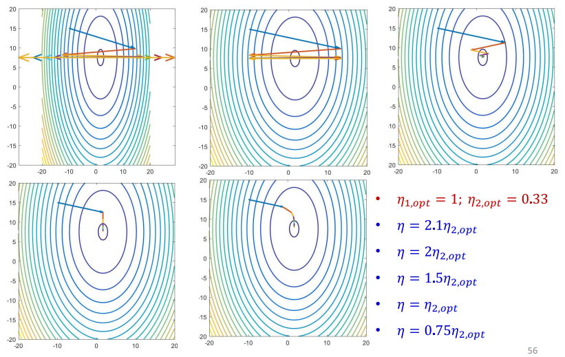
Problem with Vector Update Rule:
Conventional update applies the same step size $\eta$ to all coordinates. An issue with this is that one direction might converge optimally while another direction might diverge due to too large a step.
\[\mathbf{w}^{(k+1)} = \mathbf{w}^{(k)} - \eta \nabla_{\mathbf{w}} E\]Safe Learning Rate Rule to Avoid Divergence:
\[\eta < 2 \cdot \min_i \eta_{i,\text{opt}}\]This guarantees convergence but slows down overall learning.
Generic Convex Functions
- We can apply Taylor expansion to approximate any smooth convex function:
- $H_E$ is the Hessian of second derivatives and measures the curvature of loss function
- Optimal step size is inversely proportional to eigenvalues of the Hessian
- The eigenvalues give curvature in orthogonal directions
- For the smoothest convergence, the eigenvalues must all be equal
Convergence Challenges
- In high dimensions, convergence becomes harder to control
- Ideally, the step size $\eta$ should work for both:
- If the following condition number is large, then convergence is slow and unstable.
Decaying Learning Rate
The loss surface has many saddle points and gradient descent can stagnate on saddle points
- Start with a large learning rate to explore fast
- Gradually reduce step size to fine-tune near the minimum
- Prevents overshooting and bouncing around the optimum
Common Decay Schedules:
\[\text{Linear:} \quad \eta_k = \frac{\eta_0}{k + 1}\] \[\text{Quadratic:} \quad \eta_k = \frac{\eta_0}{(k + 1)^2}\] \[\text{Exponential:} \quad \eta_k = \eta_0 \cdot e^{-\beta k}, \quad \beta > 0\]Common Approach for Neural Networks:
- Train with a fixed learning rate until the validation loss stagnates
- Reduce learning rate:
- Resume training from the same weights, repeat as needed
RProp
- Resilient Propagation is a first-order optimization algorithm that adjusts step size independently for each parameter
- It doesn’t rely on the gradient magnitude, rather only on the sign of the gradient
- It is more robust than vanilla gradient descent
- Does not need a global learning rate
- Doesn’t require Hessian or curvature information and doesn’t assume convexity
The core idea is that at each step:
- If the gradient sign has not changed → increase step size in the same direction
- If the gradient sign has flipped → reduce step size and reverse direction (overshoot detected)
Algorithm:
- For each layer $l$, for each parameter $w_{l,i,j}$:
- While not converged:
- Update parameter:
- Recompute gradient:
Check sign consistency:
If:
\[\text{sign(prevD}(l, i, j)) == \text{sign}(D(l, i, j))\]Then,
\[\Delta w_{l, i, j} = \min(\alpha \cdot \Delta w_{l, i, j}, \Delta_{\max})\] \[\text{prevD}(l, i, j) = D(l, i, j)\]Else undo step:
\[w_{l, i, j} = w_{l, i, j} + \Delta w_{l, i, j} \quad\] \[\Delta w_{l, i, j} = \max(\beta \cdot \Delta w_{l, i, j}, \Delta_{\min})\]
QuickProp
Momentum
Incremental Stochastic Gradient Descent
| Feature | Batch Gradient Descent | Incremental Gradient Descent (SGD) |
|---|---|---|
| Update Frequency | Once per full dataset | After each training point |
| Speed per Update | Slow | Fast |
| Stability | High (smooth updates) | Noisy but flexible |
| Memory Usage | High (needs all data at once) | Low (uses one sample at a time) |
| Suitable for Big Data | Not ideal | Very efficient |
| Escaping Local Minima | Less likely | More likely (due to randomness/noise) |
Batch Gradient Descent computes gradients for all training samples and makes one big update after processing the full batch.
Incremental Gradient Descent will update one sample at a time without waiting for the full dataset.
Algorithm
- Given training data $(X_1, d_1), (X_2, d_2), \ldots, (X_T, d_T)$
- Initialize weights $W_1, W_2, \ldots, W_K \space; \space j=0$
- Repeat (over multiple epochs)
- Randomly permute $(X_1, d_1), (X_2, d_2), \ldots, (X_T, d_T)$ $\rightarrow$ stochastic
- For all $t = 1 \rightarrow T:$
- $j = j + 1$
- For each layer $k$:
- Compute Gradient $\nabla_{W_k} \text{Div}(Y_t, d_t)$
- Update weights
- Until loss converged
Important Points
- If we loop through the samples in the same order, we may get a cyclic behavior and can oscillate. We must go through them randomly to get more convergent behavior. Hence the “stochastic” nature.
- Since batch gradient descent operates over $T$ training instances to get a single update, while SGD gets $T$ updates for the same computation, the advantage of SGD is more pronounced when the data points are very similar. But as data gets increasingly diverse, the benefits of incremental update decreases, but do not entirely vanish.
- Risk of chasing the latest input: Since SGD updates the model after every point, it could swing drastically towards the latest input and never converge.
- To tackle this, we shrink the learning rate with each iteration.
- Caveat: If learning rate shrinks too much, model becomes unresponsive to new data.
- $\eta_k$ reduces with $k$ and must satisfy the conditions:
- Ensure full parameter space is explored:
- Ensure steps shrink over time:
- The fastest converging series that satisfies both above requirements is:
- If the loss is convex, SGD converges to the optimal solution. For non-convex losses, SGD converges to a local minimum.
- SGD converges faster than batch gradient descent, but arrives at a poorer optima.
Variance
Variance refers to how much our estimated loss (or error) fluctuates depending on which samples we use. When we approximate the true expected error using a finite number of training samples (empirical risk), the result is an unbiased estimate, meaning it’s correct on average, but it has variance, which affects how reliable the estimate is.
Empirical Risk Variance:
We estimate the expected divergence using:
\[\text{Loss}(W) = \frac{1}{N} \sum_{i=1}^{N} \text{div}(f(X_i; W), d_i) \\ \mathbb{E}[\text{Loss}(W)] = \mathbb{E}[\text{div}(f(X; W), g(X))]\]The variance of this estimate is:
\[\text{Var}(\text{Loss}) = \frac{1}{N} \, \text{Var}(\text{div})\]- More samples (larger $N$) → lower variance → more stable learning.
- Fewer samples → higher variance → model may learn unstable or misleading patterns.
Why Variance Matters:
- High variance means your model could “swing” wildly depending on the exact training data.
- If you only use one or two samples, the estimated error could drastically change just by replacing one data point. This affects optimization — the model might overcorrect in response to noisy updates.
In SGD:
When using Stochastic Gradient Descent, each update uses only one sample:
\[\text{div}(f(X_i; W), d_i)\]This is still an unbiased estimate of the expected error:
\[\mathbb{E}[\text{div}(f(X_i; W), d_i)] = \mathbb{E}[\text{div}(f(X; W), g(X))]\]But the variance is:
\[\text{Var}_{\text{SGD}} = \text{Var}(\text{div})\]So SGD has $N$ times more variance per update than full batch training.
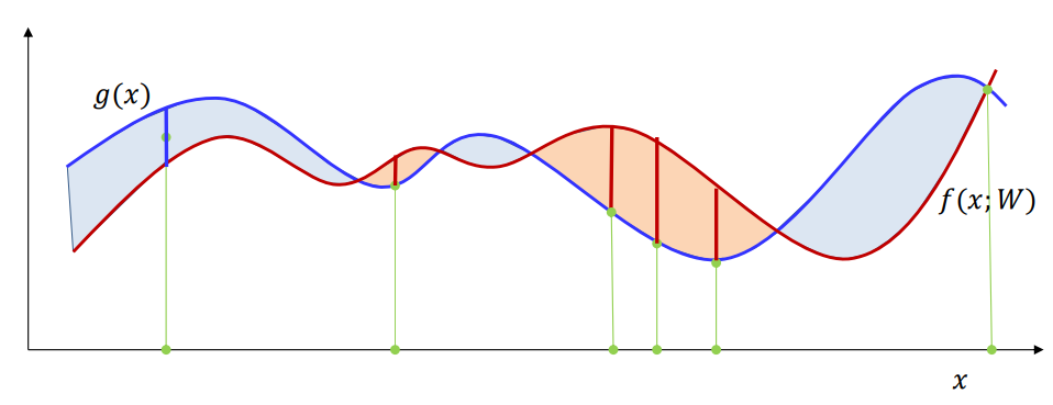
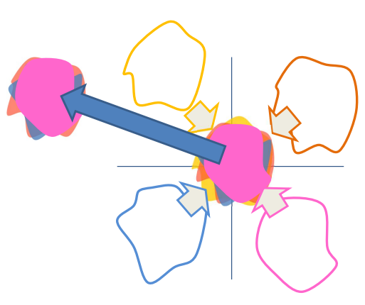
In the above image, we are trying to fit the red line to the blue line. Having more samples makes the estimate more robust to changes in the position of samples (smaller variance). But having very few samples makes the estimate swing wildly with the sample position (high variance).
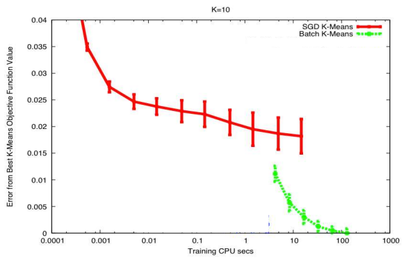
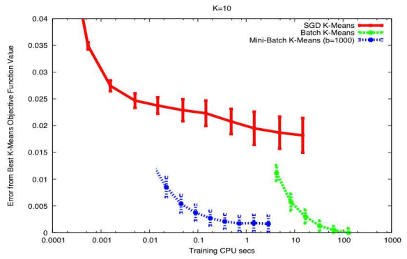
Mini-Batch Stochastic Gradient Descent
SGD uses the gradient from only one sample at a time, and is consequently high variance. But it also provides significantly quicker updates than batch gradient descent. So to get the best of both worlds, we use mini-batch incremental updates.
Algorithm
- Given training data $(X_1, d_1), (X_2, d_2), \ldots, (X_T, d_T)$
- Initialize weights $W_1, W_2, \ldots, W_K \space; \space j=0$
- Repeat (over multiple epochs)
- Randomly permute $(X_1, d_1), (X_2, d_2), \ldots, (X_T, d_T)$ $\rightarrow$ stochastic
- For all $t = 1:b:T$
- $j = j + 1$
- For each layer $k$:
- $\nabla W_k = 0$
- For $t’ = t:t+b-1$
- For every layer $k:$
- Compute Gradient $\nabla_{W_k} \text{Div}(Y_t, d_t)$
- Cumulative loss for the mini-batch:
- For every layer $k:$
- Update weights
- For every layer $k:$
- Until loss converged
Important Points
- The mini-batch size is generally set to the largest that your hardware will support (in memory) without compromising overall compute time.
- Larger minibatches implies less variance and fewer updates per epoch.
- Simple technique for convergence: fix learning rate until the error plateaus, then reduce learning rate by a fixed factor.
- Estimates have lower variance than SGD.
- Convergence rate is theoretically worse than SGD
But we compensate by being able to perform batch processing
![image.png]()
Choosing a Divergence
L2 Divergence
Used in regression
\[\text{Div} = \frac{1}{2}(y - d)^2 \\ \text{Div} = \frac{1}{2} \sum_i (y_i - d_i)^2\] \[\frac{\partial \mathcal{L}}{\partial z_k} = y_k - d_k\]KL Divergence
Used in classification tasks, especially with softmax outputs. It measures how different two probability distributions are. In classification, $Y$ is the predicted distribution and $d$ is the ground truth, usually a one-hot encoding.
\[KL(Y, d) = \sum_i d_i \log \frac{d_i}{y_i} \\ KL(Y, d) = \sum_i d_i \log(d_i) - \sum_i d_i \log(y_i)\]For one-hot, $d$ simplifies to
\[KL(Y, d) = -\log y_c\]This means that it is minimized when correct class is predicted with the highest probability $y_c \rightarrow 1$.
Gradient:
\[\frac{d}{dy_c} KL(Y, d) = -\frac{1}{y_c}\]For scalar binary classification:
\[\text{Div} = -d \log(y) - (1 - d)\log(1 - y)\]Deriving Gradient of KL Divergence with Softmax Output:
KL Divergence Loss:
\[\mathcal{L} = KL(\mathbf{d} \| \mathbf{y}) = \sum_{i=1}^C d_i \log \left( \frac{d_i}{y_i} \right)\]Softmax function:
\[y_i = \frac{e^{z_i}}{\sum_{j=1}^C e^{z_j}}\]Gradient of loss w.r.t $z_k$:
\[\frac{\partial \mathcal{L}}{\partial z_k} = - \sum_{i=1}^C d_i \cdot \frac{\partial}{\partial z_k} \log y_i\]Derivative of log-softmax:
\[\log y_i = z_i - \log \sum_j e^{z_j}\] \[\frac{\partial \log y_i}{\partial z_k} = \frac{\partial z_i}{\partial z_k} - \frac{\partial}{\partial z_k} \log \left( \sum_j e^{z_j} \right)\] \[\frac{\partial z_i}{\partial z_k} = \begin{cases}1 & \text{if } i = k \\0 & \text{if } i \neq k\end{cases}= \delta_{ik}\] \[\frac{\partial}{\partial z_k} \log \left( \sum_j e^{z_j} \right) = \frac{e^{z_k}}{\sum_j e^{z_j}} = y_k\]Therefore,
\[\frac{\partial \log y_i}{\partial z_k} = \delta_{ik} - y_k\] \[\frac{\partial \mathcal{L}}{\partial z_k} = - \sum_i d_i \left( \delta_{ik} - y_k \right) \\ = - \left( d_k (1 - y_k) + \sum_{i \ne k} d_i (-y_k) \right) = - \left( d_k - d_k y_k - y_k \sum_{i \ne k} d_i \right)\]Note that,
\[\sum_i d_i = 1 \Rightarrow \sum_{i \ne k} d_i = 1 - d_k\]So,
\[\frac{\partial \mathcal{L}}{\partial z_k} = - \left( d_k - d_k y_k - y_k (1 - d_k) \right) \\ = y_k - d_k\]Hence,
\[\frac{\partial \mathcal{L}}{\partial z_k} = y_k - d_k\]How to choose?
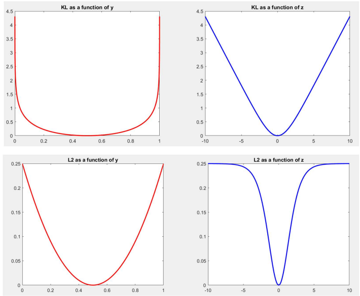
If we plot the L2 and KL divergences as a function of $y$ (one-dimensional input), we find that both are convex, and L2 appears more bowl-like and nicer compared to KL which appears to be very steep at the extremes and flatten badly near the minimum. This would show that L2 is a better divergence function for classification applications. But why do we still use KL?
Because now when we plot the divergence as a function of $z$, only the KL is nice and convex.
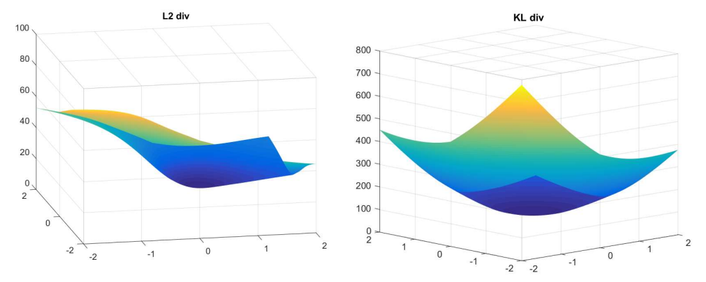
Their plots as a function of weights for a two-dimensional input look like this:
Batch Normalization
Training assumes the training data are all similarly distributed, i.e., that minibatches have similar distribution. But in practice, each minibatch may have a different distribution. So there is essentially a covariance shift and sometimes this shift could be large.
So the solution to this is to move all the minibatches to a standard location. We do this by:
- Shifting all batches to the origin by subtracting each data point in the batch with their mean
- Normalize each batch by their standard deviation
This will move the entire collection to an appropriate location and is called batch normalization.
Batch normalization is done during training and can be done independently for each unit.
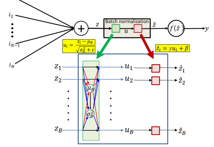
For a minibatch size $B$, we have the mean $\mu_B$ and standard deviation $\sigma_B^2$,
\[\mu_B = \frac{1}{B}\sum_{i=1}^B z_i \\ \sigma_B^2 = \frac{1}{B}\sum_{i=1}^B(z_i - \mu_B)^2\]After batch normalization,
\[u_i = \frac{z_i - \mu_B}{\sqrt{\sigma_B^2 + \epsilon}}\] \[\hat{z_i} = \gamma u_i + \beta\]where $\gamma, \beta$ are learnable parameters.
In a normal minibatch gradient descent, we compute the loss of gradients as,
\[\text{Loss(minibatch)} = \frac{1}{B}\nabla_{W_k} \text{Div}(Y_t(X_t), d_t(X_t))\]But now with batch normalization, the outputs are also functions of $\mu_B, \sigma_B^2$
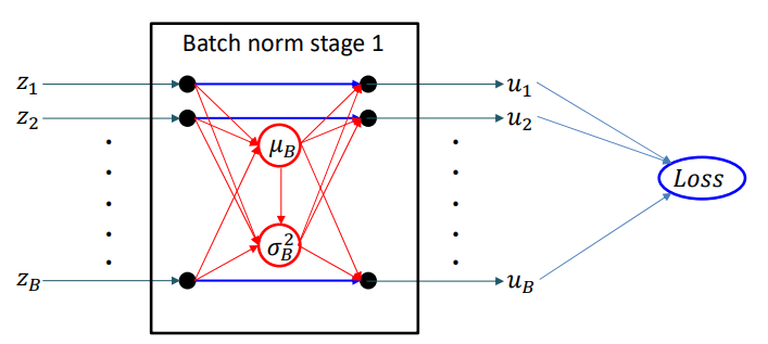
\[\text{Loss(minibatch)} = \frac{1}{B}\nabla_{W_k} \text{Div}(Y_t(X_t, \mu_B, \sigma_B^2), d_t(X_t))\]Since batch normalization is a vector function applied over all inputs from a minibatch, every $z_i$ affects every $\hat{z_j}$.
Here’s how we backpropagate,
\[\frac{dLoss}{d\hat{z}} = f'(\hat{z})\frac{dLoss}{dy}\] \[\frac{dLoss}{d\gamma} = \frac{d\hat{z}}{d\gamma}\frac{dLoss}{d\hat{z}} = u \frac{dLoss}{d\hat{z}} \\ \frac{dLoss}{d\beta} = \frac{d\hat{z}}{d\beta}\frac{dLoss}{d\hat{z}} = \frac{dLoss}{d\hat{z}}\] \[\frac{dLoss}{du_i} = \frac{d\hat{z_i}}{du_i}\frac{dLoss}{d\hat{z_i}} = \gamma \frac{dLoss}{d\hat{z_i}}\]Now we need to compute $\frac{dLoss}{du_i}$ for every $u_i$.
The complete derivative of the mini-batch loss w.r.t. $z_i$
\[\frac{dLoss}{dz_i} = \sum_j\frac{dLoss}{du_j}\frac{du_j}{dz_i}\]The first part of this has been computed above. We now need to compute $\frac{du_i}{dz_i}$ for every pair $i,j$.
First when $i=j$,
\[\frac{du_i}{dz_i} = \frac{\partial u_i}{\partial z_i} + \frac{\partial u_i}{\partial \mu_B}\frac{\partial \mu_B}{\partial z_i} + \frac{\partial u_i}{\partial \sigma_B^2}\frac{d \sigma_B^2}{d z_i}\]First term:
\[\frac{\partial u_i}{\partial z_i} = \frac{1}{\sqrt{\sigma_B^2 + \epsilon}}\]Second term:
\[\frac{\partial u_i}{\partial \mu_B} = \frac{-1}{\sqrt{\sigma_B^2 + \epsilon}} \\ \frac{\partial \mu_B}{\partial z_i} = \frac{1}{B}\]Third term:
\[\frac{\partial u_i}{\partial \sigma_B^2} = \frac{-(z_i - \mu_B)}{2(\sigma_B^2 + \epsilon)^{3/2}}\] \[\frac{d \sigma_B^2}{dz_i} = \frac{\partial d\sigma_B^2}{\partial z_i} + \frac{\partial \sigma_B^2}{\partial \mu_B}\frac{\partial \mu_B}{\partial z_i}\] \[\frac{\partial \sigma_B^2}{\partial z_i} = \frac{2(z_i - \mu_B)}{B} \\ \frac{\partial \sigma_B^2}{\partial \mu_B} = 0\] \[\frac{\partial u_i}{\partial \sigma_B^2} \cdot \frac{\partial \sigma_B^2}{\partial z_i} = \frac{-(z_i - \mu_B)}{2(\sigma_B^2 + \epsilon)^{3/2}} \cdot \frac{2(z_i - \mu_B)}{B} \\ = \frac{-(z_i - \mu_B)^2}{B(\sigma_B^2 + \epsilon)^{3/2}}\]So, for $i=j$,
\[\frac{d u_i}{d z_i} = \frac{1}{\sqrt{\sigma_B^2 + \epsilon}} + \frac{-1}{B \sqrt{\sigma_B^2 + \epsilon}} + \frac{-(z_i - \mu_B)^2}{B(\sigma_B^2 + \epsilon)^{3/2}}\]Now when $i \neq j$,
\[\frac{d u_j}{d z_i} = \frac{\partial u_j}{\partial \mu_B} \frac{\partial \mu_B}{\partial z_i} + \frac{\partial u_j}{\partial \sigma_B^2} \frac{\partial \sigma_B^2}{\partial z_i}\]This is similar to the case when $i=j$ but without the first term. So,
\[\frac{d u_j}{d z_i} = \frac{-1}{B \sqrt{\sigma_B^2 + \epsilon}} + \frac{-(z_i - \mu_B)(z_j - \mu_B)}{B(\sigma_B^2 + \epsilon)^{3/2}}\]Full derivative summary:
\[\frac{d u_j}{d z_i} =\begin{cases}\frac{1}{\sqrt{\sigma_B^2 + \epsilon}} + \frac{-1}{B \sqrt{\sigma_B^2 + \epsilon}} + \frac{-(z_i - \mu_B)^2}{B(\sigma_B^2 + \epsilon)^{3/2}} & \text{if } i = j \\\frac{-1}{B \sqrt{\sigma_B^2 + \epsilon}} + \frac{-(z_i - \mu_B)(z_j - \mu_B)}{B(\sigma_B^2 + \epsilon)^{3/2}} & \text{if } i \ne j\end{cases}\] \[\frac{dLoss}{dz_i} = \sum_j\frac{dLoss}{du_j}\frac{du_j}{dz_i}\] \[\frac{d \mathcal{L}}{d z_i} = \frac{1}{\sqrt{\sigma_B^2 + \epsilon}} \cdot \frac{d \mathcal{L}}{d u_i} + \frac{-1}{B \sqrt{\sigma_B^2 + \epsilon}} \sum_j \frac{d \mathcal{L}}{d u_j} + \frac{-(z_i - \mu_B)}{B(\sigma_B^2 + \epsilon)^{3/2}} \sum_j \frac{d \mathcal{L}}{d u_j} (z_j - \mu_B)\]The rest of the backpropagation continues normally from $\frac{d \mathcal{L}}{d z_i}$
Inference
On test data, we still do batch normalization. But don’t have minibatches and we perform inference over individual instances. So we will use the average over all training batches, as follows:
\[\mu_{BN} = \frac{1} \sum_{batch} \mu_B({batch})\] \[\sigma_{BN}^2 = \frac{B}{(B-1){Nbatches}} \sum_{batch} \sigma_B^2({batch})\]$\mu_B(batch), \sigma_B^2(batch)$ are obtained from the final converged network.
Important Points
- Batch normalization may only be applied to some layers or even only selected neurons in a layer
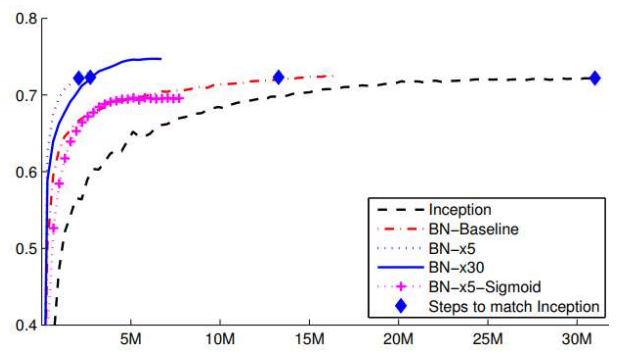
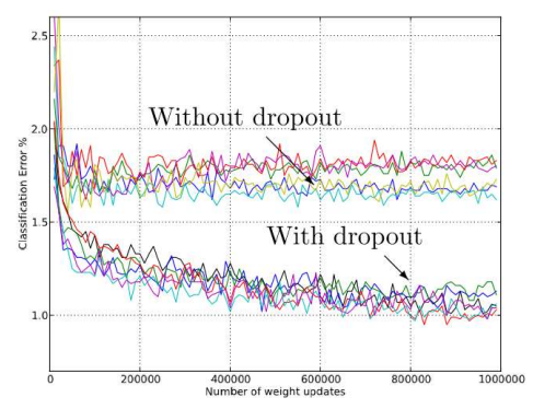
- Improves both convergence rate and neural network performance
- Anecdotal evidence suggests that BN eliminates the need for dropout
- To get maximum benefit from BN, learning rates must be increased and learning rate decay can be faster
- Also needs better randomization of training data order
Regularization
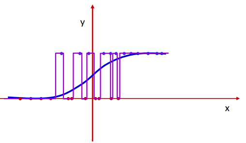
For a simple binary classifier, the desired output would be the smooth blue curve. But the perceptron network is also fully capable of learning the purple curve. This is because the perceptrons in the network are individually capable of sharp changes in output.
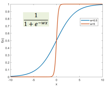
If you consider a sigmoid activation function, the function becomes steeper with increasing magnitude of weights. So the model can fully learn large weights so that the output has steep edges.
So the solution to preventing this is contrain the weights $w$ to be low, which will force perceptrons to learn slowly and give a smoother output response.
Regularized training loss:
\[L(W_1, W_2, \ldots, W_K) = \frac{1}{T} \sum_t \text{Div}(Y_t, d_t) + \frac{1}{2} \lambda \sum_k \| W_k \|_F^2\]Batch Mode Gradient:
\[\nabla_{W_k} L = \frac{1}{T} \sum_t \nabla_{W_k} \text{Div}(Y_t, d_t) + \lambda W_k^T\]Stochastic Gradient Descent:
\[\nabla_{W_k} L = \nabla_{W_k} \text{Div}(Y_t, d_t) + \lambda W_k^T\]Mini-batch Gradient:
\[\nabla_{W_k} L = \frac{1}{b} \sum_{\tau = t}^{t + b - 1} \nabla_{W_k} \text{Div}(Y_{\tau}, d_{\tau}) + \lambda W_k^T\]Weight update:
\[W_k \leftarrow (1 - \lambda) W_k - \eta \frac{1}{b} \sum_{\tau = t}^{t + b - 1} \nabla_{W_k} \text{Div}(Y_{\tau}, d_{\tau})\]$\lambda$ gives a measure of how important it is to prioritize regularization.
Important Points
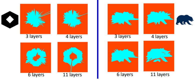
- For a given number of parameters, deeper networks impose more smoothness than shallow ones. This is because each layer works on the already smooth surface output by the previous layer.
- Data underspecification can result in overfitted models and must be handled by regularization and more constrained (generally deeper) network architectures
Dropout
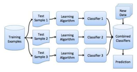
Bagging:
- This is a method that samples training data and trains several different classifiers
- Then we classify the test instances with the entire ensemble of classifiers, after which we vote across classifiers for final decision
- It is empirically shown to improve significantly over training a single classifier from combined data
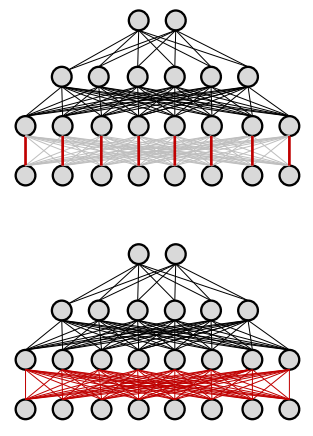
In dropout, during training for each input, for every iteration, we turn of each neuron with a probability $1-\alpha$. In practice, set them to 0 according to the failure of a Bernoulli random number generator with success probability $\alpha$. Backpropagation is effectively performed only over the remaining network.
So each training instance or epoch, essentially sees a different training network.
Statistical interpretation:
- For a network with a total $N$ neurons, there are $2^N$ possible sub-networks obtained by randomly turning on and off the neurons.
- Since $2^N$ is a very large number, dropout samples over all these possible networks.
- Then by bagging, we learn a network that averages over all possible networks.
Another interpretation:
- In a rich and dense network, there is nothing stopping the network from learning a pass-through, i.e., just cloning the input to its output. Because of this, we would essentially lose the neuron and maybe a whole layer.
- Dropout forces the neurons to learn denser patterns.
Algorithm
Forward Pass:
- Given inputs $\mathbf{x} = [x_j, \quad j = 1 \ldots D]$
- Set:
- $D_0 = D$, is the width of the $0^{th}$ (input) layer
- $y_j^{(0)} = x_j, \quad j = 1 \ldots D$
- $y_0^{(k=1\ldots N)} = x_0 = 1$
- For layers $k = 1 \ldots N$
- Apply dropout mask: $\text{mask}(k - 1, j) = \text{Bernoulli}(\alpha), \quad j = 1 \ldots D_{k-1}$
- $\tilde{y}j^{(k-1)} = y_j^{(k-1)} \cdot \text{mask}(k - 1, j), \quad j = 1 \ldots D{k-1}$
For each neuron $j = 1 \ldots D_k$:
\[z_j^{(k)} = \sum_{i=0}^{D_{k-1}} w_{ij}^{(k)} \cdot \tilde{y}_i^{(k-1)} + b_j^{(k)}\] \[y_j^{(k)} = f_k \left( z_j^{(k)} \right)\]
- Output: $Y = y_j^{(N)}, \quad j = 1 \ldots D_N$
Backward Pass:
- Output layer $(k=N)$:
- For layers $k = (N-1) \ldots 0$:
For each neuron $i = 1 \ldots D_k$:
\[\frac{\partial \text{Div}}{\partial y_i^{(k)}} = \text{mask}(k, i) \cdot \sum_j w_{ij}^{(k+1)} \cdot \frac{\partial \text{Div}}{\partial z_j^{(k+1)}}\] \[\frac{\partial \text{Div}}{\partial z_i^{(k)}} = f_k' \left( z_i^{(k)} \right) \cdot \frac{\partial \text{Div}}{\partial y_i^{(k)}}\] \[\frac{\partial \text{Div}}{\partial w_{ij}^{(k+1)}} = y_i^{(k)} \cdot \frac{\partial \text{Div}}{\partial z_j^{(k+1)}}\]
Inference:
- Given inputs $\mathbf{x} = [x_j, \quad j = 1 \ldots D]$
- Set:
- $D_0 = D$, is the width of the $0^{th}$ (input) layer
- $y_j^{(0)} = x_j, \quad j = 1 \ldots D$
- $y_0^{(k=1\ldots N)} = x_0 = 1$
- For layers $k = 1 \ldots N$
For each neuron $j = 1 \ldots D_k$:
\[z_j^{(k)} = \sum_{i=0}^{D_{k-1}} w_{ij}^{(k)} \cdot {y}_i^{(k-1)} + b_j^{(k)}\] \[y_j^{(k)} = \alpha f_k \left( z_j^{(k)} \right)\]
- Output: $Y = y_j^{(N)}, \quad j = 1 \ldots D_N$
Exploding & Vanishing Gradients
A Multilayer Perceptron (MLP) with multiple hidden layers is essentially a nested composition of functions:
\[Y = f_N\left(W_N f_{N-1}\left(W_{N-1} \cdots f_1(W_1 X) \right) \right)\]We define the error or divergence on the output prediction as:
\[Div(X) = D\left(f_N\left(W_N f_{N-1}\left(W_{N-1} \cdots f_1(W_1 X) \right) \right)\right)\]To perform backpropagation through this nested structure, we compute the gradient of the divergence with respect to the output of each hidden layer:
\[\nabla_{f_k} Div = \nabla D \cdot \nabla f_N \cdot W_N \cdot \nabla f_{N-1} \cdot W_{N-1} \cdots \nabla f_{k+1} \cdot W_{k+1}\]Why Deep Networks are Hard to Train
The challenge arises because of repeated multiplication of Jacobian matrices during backpropagation:
- For typical activations like ReLU, sigmoid, tanh:
- The Jacobian is a diagonal matrix.
Each diagonal entry is the derivative of the activation, i.e., $f’_k(z_i)$
\[\nabla f_k(z) =\begin{bmatrix}f_k'(z_1) & 0 & \cdots & 0 \\0 & f_k'(z_2) & \cdots & 0 \\\vdots & \vdots & \ddots & \vdots \\0 & 0 & \cdots & f_k'(z_n)\end{bmatrix}\]
- These derivatives are typically $<1$
- Hence, multiplying by Jacobians shrinks the gradient at each layer
- So after a few layers, the derivative of the divergence at any time is totally forgotten
Effect of weights:
Each weight matrix $W_n$ performs a linear transformation of the gradient. Specifically:
- It scales the gradient in different directions.
- The amount of scaling is determined by the singular values (or eigenvalues for symmetric matrices) of the matrix.
Let’s say the singular values of a matrix $W_n$ are $\sigma_1, \sigma_2, \ldots, \sigma_m$
- If all $\sigma_i<1 \rightarrow$ gradient will shrink in all directions
- If any $\sigma_i > 1 \rightarrow$ gradient may grow in that direction
If many weight matrices have singular values greater than 1, then the gradients will explode.
If many weight matrices have singular values lesser than 1, then the gradients will vanish.