Analysis of Battery in Low Power Electric Vehicles using Machine Learning

The following project has been done as part of my Practice School-1 cirriculum under CSIR - Central Electronics Engineering Research Institute (CEERI), Pilani. It enabled me to work on real-world issues and provided me with an opportunity to obtain industrial experience under the guidance of Dr. Bhausaheb Ashok Botre, Principal Scientist.

Abstract

Due to its numerous favorable effects on the environment and society, electric vehicles (EVs) are growing in popularity around the world. This Project Report discusses the use of Machine Learning techniques for the analysis of batteries in low power Electric-tricycle. The report talks about the use of machine learning techniques such as Random Forest (RF) and Gradient Boosting Regression Tree (GBRT) for State of Charge (SOC) estimation and load forecasting. MATLAB simulations for speed control of a BLDC motor using PID controller and a Lithium-ion temperature dependent battery model are used to predict the SOC and the power of the battery. The data generated from these simulations is used to train the ML models.

Project Areas: Electric Vehicles, Machine Learning.

Keywords: Machine Learning, State of Charge, BMS, Load Forecasting, BLDC motor.

Introduction

Electric Vehicles are becoming increasingly integrated in several cities. With increasing EV technology and smart power grids, they have emerged as an alternative to the conventional gas driven vehicles. Being more environmentally friendly, people are rapidly moving towards EVs.

Battery charging in EVs is still a major challenge and continuous research efforts are being made to build an efficient system to analyze the various parameters of the batteries being used. Accurate analysis needs to be performed to prevent any battery failure and occurrence of any accidents.

Problem Statement

The aim of this project is to analyze batteries in low power Electric Vehicles using Machine Learning techniques. CEERI Pilani has developed an electric assisted tricycle for the outdoor mobility of differently abled persons and aims to improve it by incorporating an efficient Battery Management System using IoT and ML techniques.

Challenges Addressed

A number of challenges are involved in analyzing the batteries of Electric Vehicles, which include:

1. Prediction of driving range
2. Performance of battery
3. Charge load conditions
4. State of charge (SOC) estimation

The absence of high-quality, full-scale datasets is one of the most critical challenges faced in the accurate prediction of batteries in EVs. But in recent times, one major starting point in the prediction of battery safety is the simulation of the loading conditions. My personal objective is to focus on the EV load conditions and SOC estimation techniques to help build an efficient battery management system (BMS).

Analysis of EV charge load conditions implies analyzing the power of the battery during peak demands. It also looks at how charging the EV affects the battery. It is important because EV load balancing instructs the chargers to deliver the right amount of energy and manages the energy flow. So analyzing the energy trends of the battery would tell us its charge load characteristics.

The most critical inputs for controlling EV charging and improving power system operation and performance are accurate early knowledge of the EV load demand. Moreover, factors such as driving and travel patterns of each EV lead to a stochastic nature of the EV charging demand.

SOC is a number between 0 and 1 that indicates the amount of charge available in the cell relative to the maximum amount of charge. A major challenge with SOC is that it cannot be measured directly but it needs to be inferred based on measurements of voltage, current, temperature and the use of a model of the cell. However, some Simulink models of batteries let us obtain SOC data directly which is extremely beneficial.

Machine Learning

There exist a number of traditional techniques for EV load analysis and SOC estimation. But most of them have been proved less efficient in recent times, and with the rise of machine learning, we have a lot more options to help in load forecasting and SOC estimation.

A popular way of modeling batteries with the purpose of system design and charge load analysis is to create an electro-thermal analogy for the cell’s behavior, i.e, to create an equivalent circuit. The topology and parameters of the equivalent circuit should allow us to load it in the same way we would load a battery and observe the same response a battery would have. This includes voltage drop, relaxation times and open circuit voltage, as functions of temperature and state of charge (SOC).

The easiest way to estimate SOC is integrating current. It is a computationally cheap method but the disadvantage is that any error in the measurement of current will accumulate over time, making the SOC diverge from its true value.

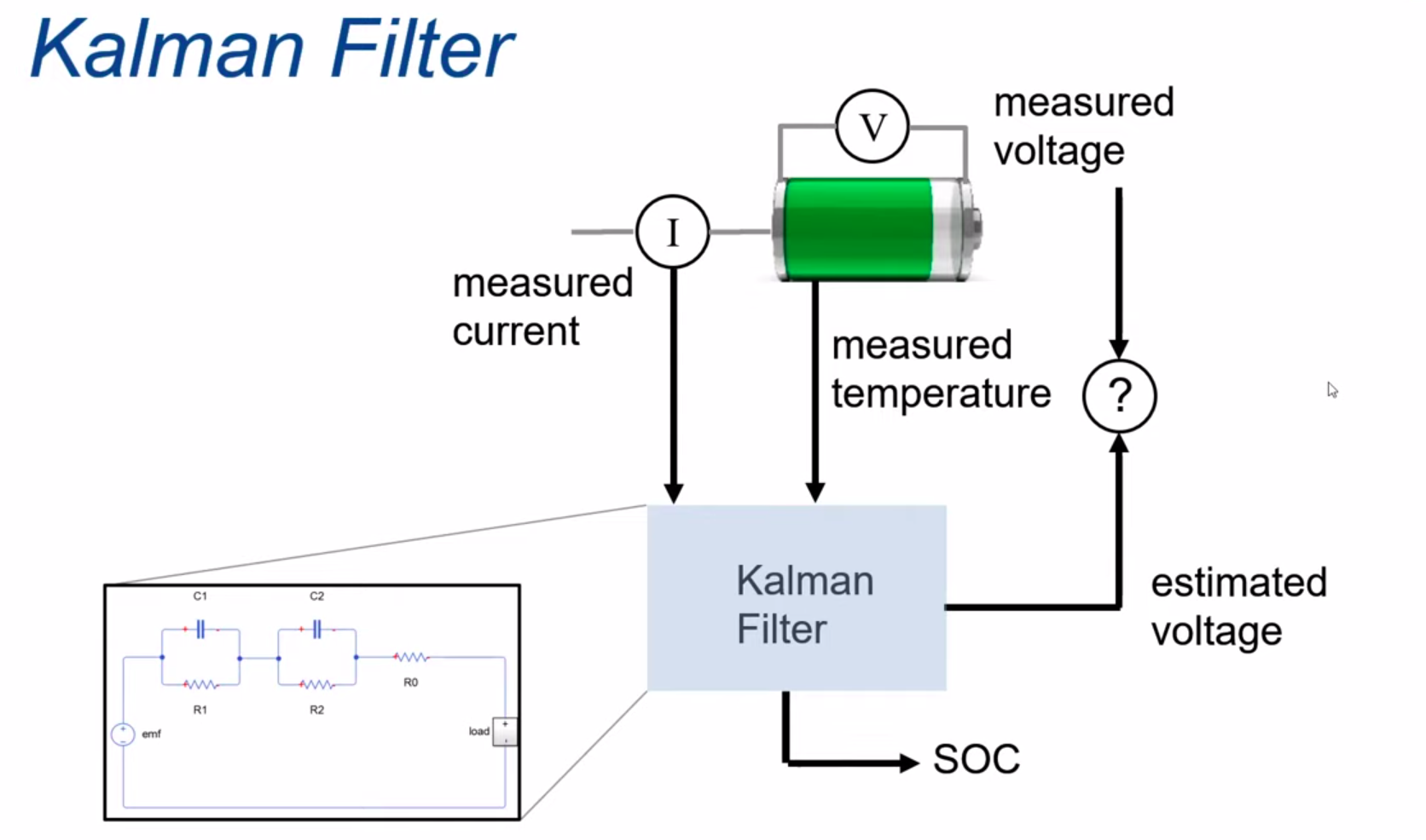
A more advanced method of estimating SOC is the use of observers such as Kalman filters. The Kalman filter takes in the model of the cell and uses a recursive algorithm that continuously predicts a future state and corrects it using measurements performed on the system. But this is computationally very expensive.

An alternative would be to use Machine Learning models that take the relevant parameters and use them to predict the desired features. Trained with a sufficiently large amount of data measured under sufficiently varied conditions, ML models would be able to learn the patterns of change in the measurable quantities of the battery and link them to predict the SOC and power/energy trends.

Machine learning algorithms provide a variety of approaches for forecasting EV load conditions and SOC estimation. Random Forest (RF) and Gradient Boosting Regression Tree (GBRT) are two such techniques that have lately proven to be useful.

Random Forest (RF):

The Random Forest algorithm is based on decision trees. A decision tree is a model that follows a path from the branched observations to the outcomes. We use regression trees since the outcomes (power/energy consumption and SOC) have continuous values.

Random Forest Regression is a supervised learning approach for regression that employs ensemble learning methods. Ensemble learning method is a technique that combines predictions from multiple machine learning algorithms to make a more accurate prediction than a single model.

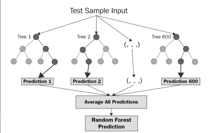
The diagram above shows the structure of a RF. The trees run in parallel with no interaction amongst them. An RF operates by constructing several decision trees during training time and outputting the mean of the classes as the prediction of all the trees.

Random Forest Regression is a powerful and precise model. It usually works well on a wide range of issues, including those with non-linear relationships.

Gradient Boosting Regression Tree (GBRT):

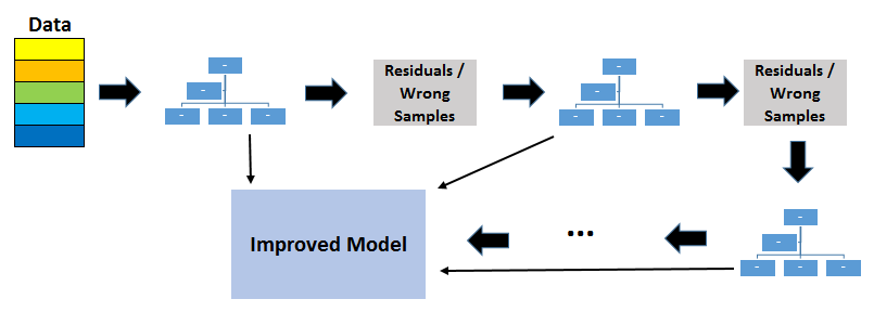
GBRT is also based on decision trees and ensemble learning. It also works on the concept of Boosting, which works on the principle of improving mistakes of the previous learner through the next learner. In boosting, weak learners are used which perform only slightly better than a random chance.

In GBRT, we combine many weak learners to come up with one strong learner. The weak learners here are the individual decision trees. All the trees are connected in series and each tree tries to minimize the error of the previous tree. Due to this sequential connection, boosting algorithms are usually slow to learn, but also highly accurate.

Overfitting owing to the inclusion of too many trees is a problem that we may face in GBRT but not in Random Forests. Overfitting will not occur in RF if you add too many trees. Although the model’s accuracy does not improve after a certain point, there is no issue with overfitting. However, when using GBRT, we must be cautious about the amount of trees we choose, as having too many weak learners in the model can lead to data overfitting. As a result, hyperparameter optimization is quite important.

Simulations

MATLAB is a great software platform that provides us with a number of tools that can be used to model an EV system. Two Simulink models were created to obtain data used for SOC estimation and load forecasting.

1. Lithium-Ion Temperature Dependent Battery Model
2. Speed Control of a BLDC Motor using PID Controller

These two individual models were then interfaced together to create a single large model that predicts SOC and power trends in the presence of a BLDC motor as load.

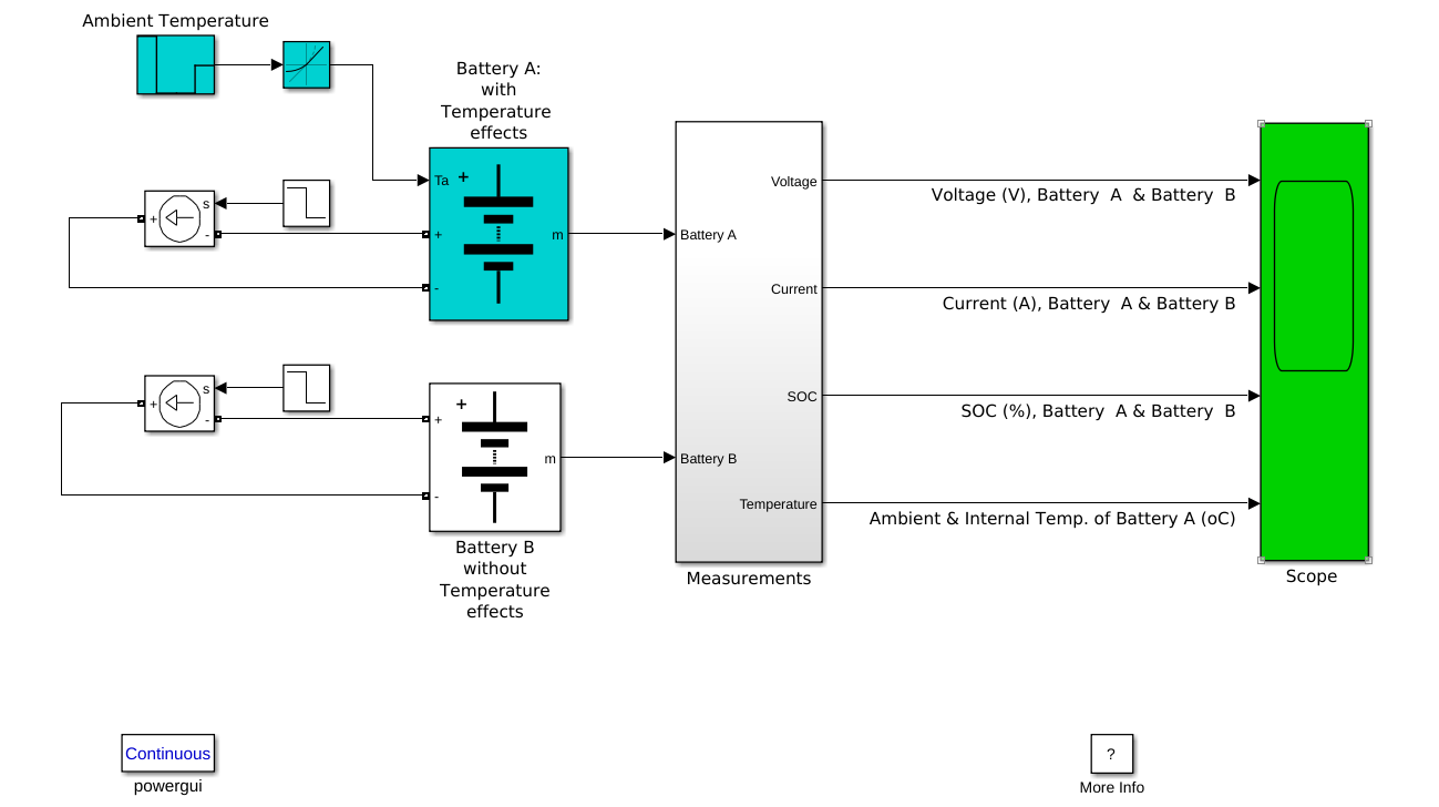
Lithium-Ion Temperature Dependent Battery Model

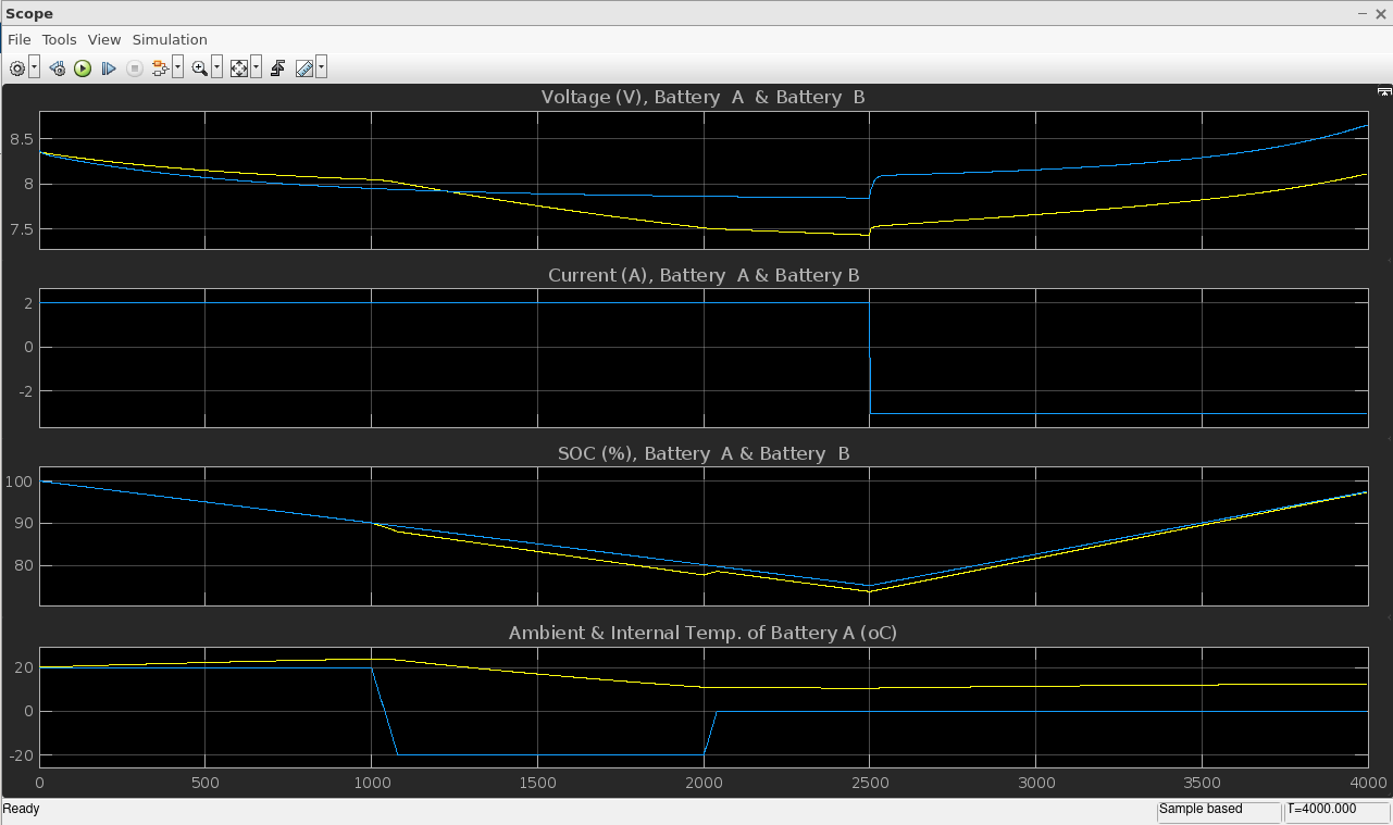
This model shows the variation in performance of a 7.2 V, 5.4 Ah Lithium-Ion battery. Throughout a discharge and charge operation, the model is exposed to an environment with varying ambient temperature. Its performance is contrasted with the scenario in which temperature effects are disregarded. The temperature dependent battery model functions reasonably well, as seen from the scope. The output voltage and capacity change together with the cell’s internal temperature as a result of charge (or discharge) heat losses and variations in the outside temperature.

The data from the scope can be extracted into an excel sheet, as shown below, containing all the necessary parameters. By using data of only the relevant parameters, ML models can be trained to estimate the SOC and power trends (for load forecasting).

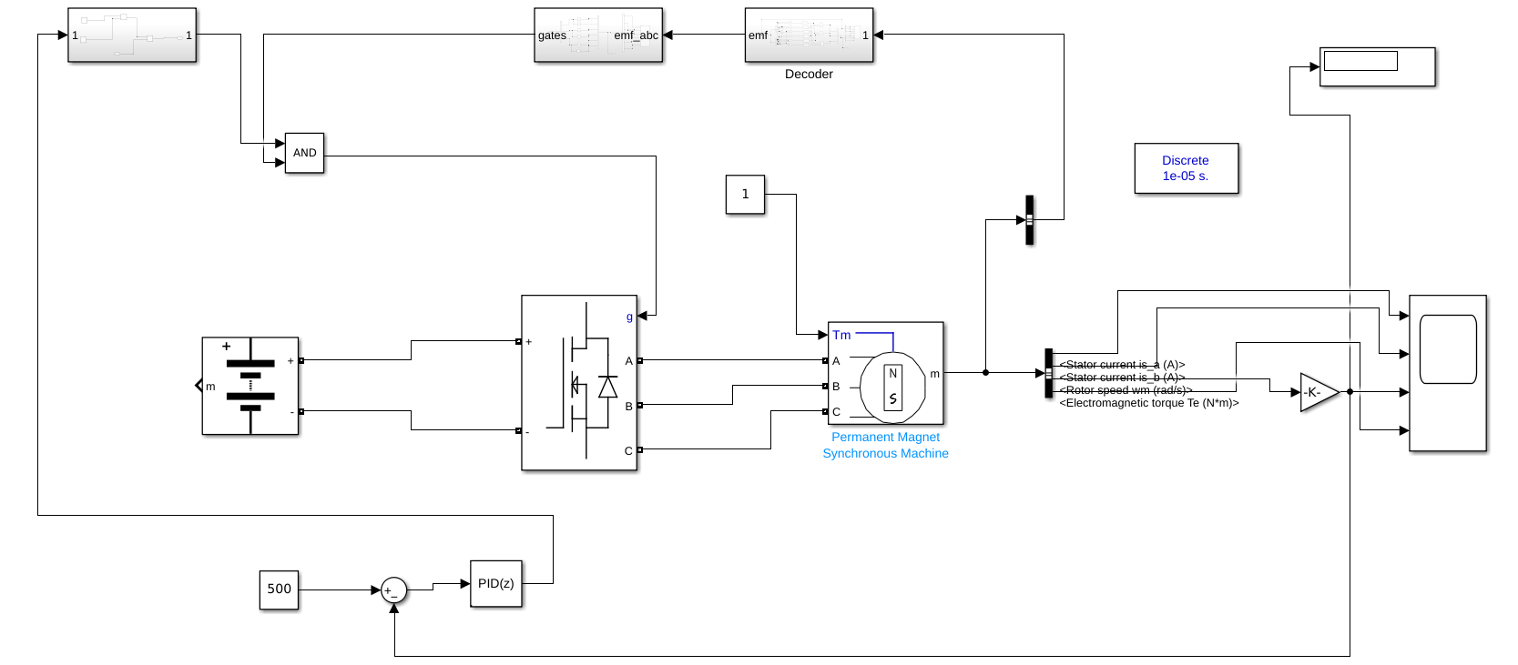
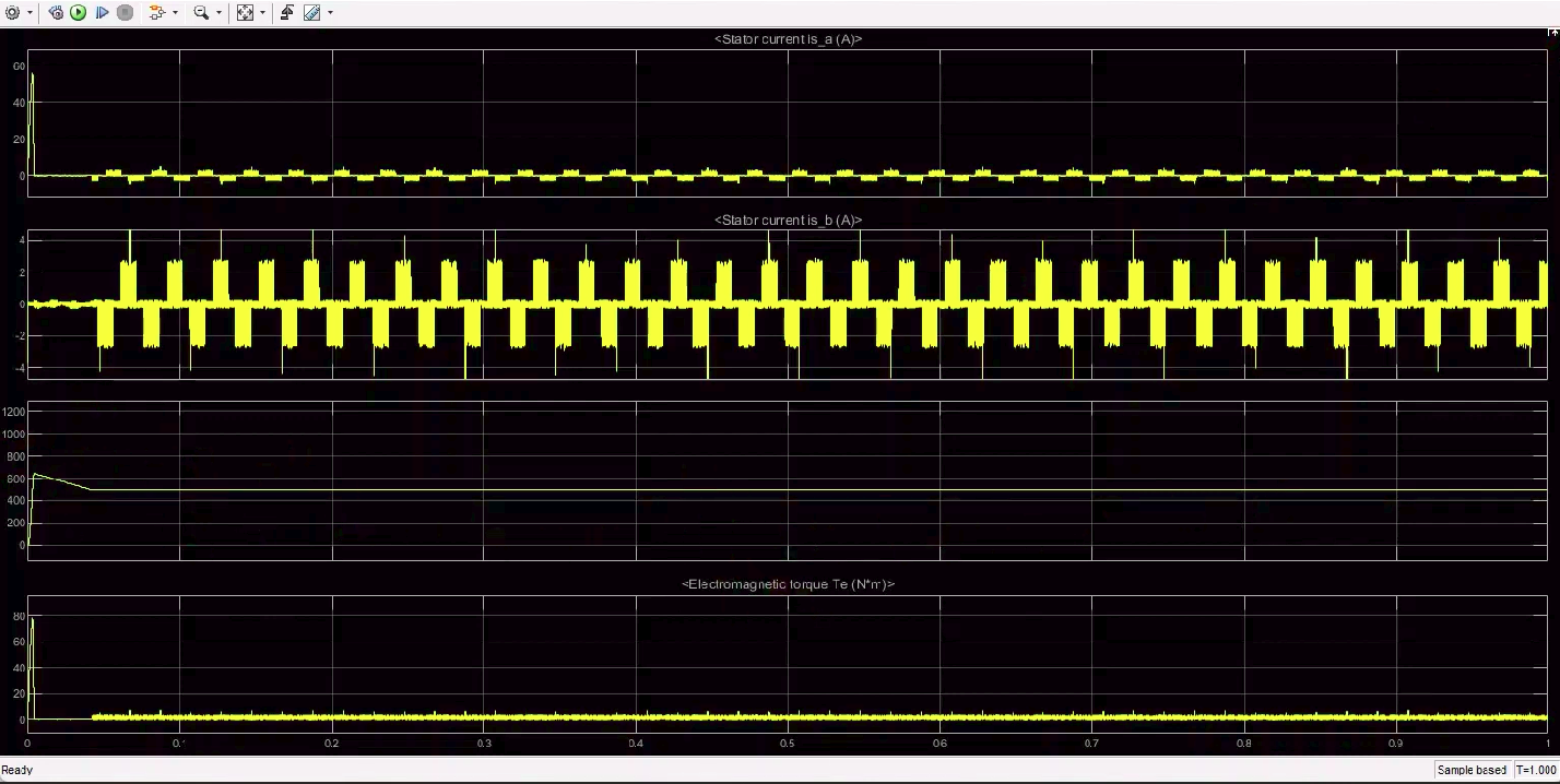
Speed Control of a BLDC Motor using PID Controller

This model displays the functionality of a Brushless DC motor coupled to a PID controller for precision and stability. Ignoring the effects of temperature, a Lithium-Ion battery is connected to the motor. We use the scope to monitor changes in stator currents, motor speed, and electromagnetic torque. The PID controller ensures that the motor’s speed is consistently maintained at the required rpm specified in the input.

Complete Model

The two models generated above are combined to obtain one single large model. This demo shows the performance of the Lithium-Ion battery in the presence of a load, i.e., BLDC motor, its variation with change in temperature and allows us to measure motor speed as well.

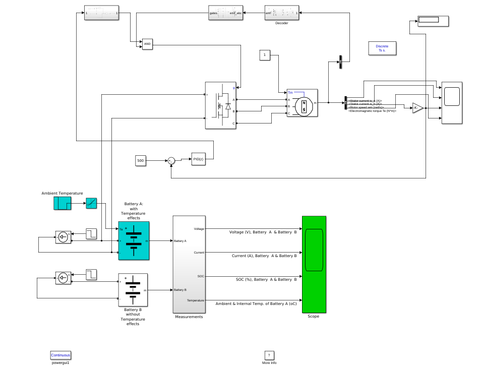
The information from the scope can be retrieved into an excel file that includes all the relevant parameters. This complete data can then be used to train the ML models that will accurately predict the SOC and the power/energy consumed for load forecasting.

Results

The complete MATLAB simulation, however, is extremely heavy and time consuming, and requires higher specs and computational power to run. So the ML models were trained based on data generated from the battery without the presence of a load.

Datasets

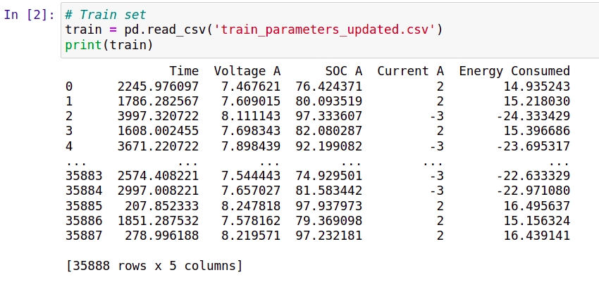
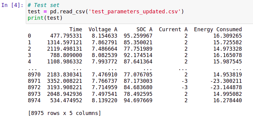
The data obtained from the MATLAB simulation in an excel sheet is shuffled randomly and divided into training sets and testing sets.

Random Forest

Scikit learn library is used to run the Random Forest model and is trained on the training dataset. The trained model is then tested on the test dataset and the accuracy is measured.

Code:

# Importing the libraries
import numpy as np
import matplotlib.pyplot as plt
import pandas as pd

# Train set
train = pd.read_csv('train_parameters_updated.csv')

energy = train.iloc[:,4].values
soc = train.iloc[:,2:3].values 
time = train.iloc[:,0:1].values # X

# Test set
test = pd.read_csv('test_parameters_updated.csv')

energy_test = test.iloc[:,4].values
soc_test = test.iloc[:,2:3].values 
time_test = test.iloc[:,0:1].values # X

# Predict SOC
from sklearn.ensemble import RandomForestRegressor
regressor_1 = RandomForestRegressor(n_estimators = 10, random_state = 0)
regressor_1.fit(time,soc)

# Visualizing the SOC Set 
X_grid = np.arange(min(time), max(time), 0.01)
X_grid = X_grid.reshape((len(X_grid), 1))
plt.scatter(time_test, soc_pred, color = 'red')
plt.plot(X_grid, regressor_1.predict(X_grid), color = 'blue')
plt.title('Random Forest Regression')
plt.xlabel('Time')
plt.ylabel('SOC')
plt.show()

# Predict Energy
from sklearn.ensemble import RandomForestRegressor
regressor_2 = RandomForestRegressor(n_estimators = 10, random_state = 0)
regressor_2.fit(time,energy)

energy_pred = regressor_2.predict(time_test)

# Visualizing the Energy Set 
X_grid = np.arange(min(time), max(time), 0.01)
X_grid = X_grid.reshape((len(X_grid), 1))
plt.scatter(time_test, energy_pred, color = 'red')
plt.plot(X_grid, regressor_2.predict(X_grid), color = 'blue')
plt.title('Random Forest Regression')
plt.xlabel('Time')
plt.ylabel('Energy')
plt.show()

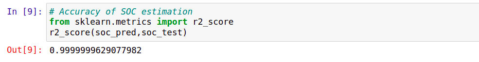
# Accuracy of SOC estimation
from sklearn.metrics import r2_score
r2_score(soc_pred,soc_test)

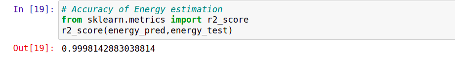
# Accuracy of Energy estimation
from sklearn.metrics import r2_score
r2_score(energy_pred,energy_test)

Predicting SOC:

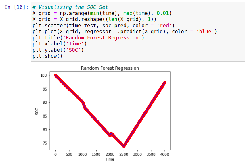
Accuracy: 99%

Predicting Energy:

The data for energy is obtained by multiplying the voltage and the current. The trends in energy are used for load forecasting.

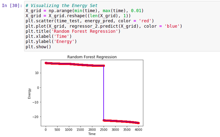
Accuracy: 99%

Model Summary:

import sklearn.metrics as metrics

mae = metrics.mean_absolute_error(soc_test, soc_pred)
mse = metrics.mean_squared_error(soc_test, soc_pred)
rmse = np.sqrt(mse) # or mse**(0.5)  
r2 = metrics.r2_score(soc_test,soc_pred)

print("Results of sklearn.metrics:")
print("MAE:",mae)
print("MSE:", mse)
print("RMSE:", rmse)
print("R-Squared:", r2)

mae = metrics.mean_absolute_error(energy_test, energy_pred)
mse = metrics.mean_squared_error(energy_test, energy_pred)
rmse = np.sqrt(mse) # or mse**(0.5)  
r2 = metrics.r2_score(energy_test,energy_pred)

print("Results of sklearn.metrics:")
print("MAE:",mae)
print("MSE:", mse)
print("RMSE:", rmse)
print("R-Squared:", r2)

For SOC: MAE: 0.0007033089960029275 MSE: 7.885088251654824e-07 RMSE: 0.0008879801941290596 R-Squared: 0.9999999861769471

For Energy: MAE: 0.0042136681167083585 MSE: 0.15557361977356302 RMSE: 0.3944282187845629 R-Squared: 0.9995374972380205

Gradient Boosting Regression Tree

This model also uses the Scikit learn library to train the model on the training data. The trained model is then tested on the test dataset and the accuracy is measured.

Code:

# Load libraries
from sklearn.ensemble import GradientBoostingRegressor
import numpy as np
import pandas as pd
from sklearn.model_selection import train_test_split
from sklearn.metrics import mean_squared_error
from sklearn.metrics import mean_absolute_error
from sklearn.metrics import r2_score
import warnings
warnings.filterwarnings('ignore')

# Train set
data = pd.read_csv('train_parameters_updated.csv')

energy = data.iloc[:,4].values
soc = data.iloc[:,2:3].values 
time = data.iloc[:,0:1].values # X

gradientregressor = GradientBoostingRegressor(max_depth=2,n_estimators=3,learning_rate=1.0)

# Test set
test = pd.read_csv('test_parameters_updated.csv')

energy_test = test.iloc[:,4].values
soc_test = test.iloc[:,2:3].values 
time_test = test.iloc[:,0:1].values # X

# Predict SOC
model = gradientregressor.fit(time,soc)
soc_pred = model.predict(time_test)

# Visualizing the SOC Set 
import matplotlib.pyplot as plt
%matplotlib inline

X_grid = np.arange(min(time), max(time), 0.01)
X_grid = X_grid.reshape((len(X_grid), 1))
plt.scatter(time, soc, color = 'red')
plt.title('GBRT')
plt.xlabel('Time')
plt.ylabel('SOC')
plt.show()

# Predict Energy
model_2 = gradientregressor.fit(time,energy)
energy_pred = model_2.predict(time_test)

# Visualizing the Voltage Set 
import matplotlib.pyplot as plt
%matplotlib inline

X_grid = np.arange(min(time), max(time), 0.01)
X_grid = X_grid.reshape((len(X_grid), 1))
plt.scatter(time_test, energy_pred, color = 'red')
plt.plot(X_grid, model_2.predict(X_grid), color = 'blue')
plt.title('GBRT')
plt.xlabel('Time')
plt.ylabel('Energy')
plt.show()

# Accuracy of SOC estimation
r2_score(soc_pred,soc_test)

# Accuracy of Energy estimation
r2_score(energy_pred,energy_test)

Predicting SOC:

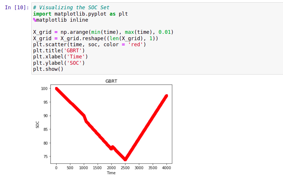
Accuracy: 93%

Predicting Energy:

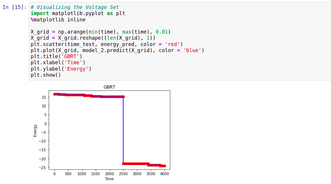
Accuracy: 99%

Model Summary:

import sklearn.metrics as metrics

mae = metrics.mean_absolute_error(soc_test, soc_pred)
mse = metrics.mean_squared_error(soc_test, soc_pred)
rmse = np.sqrt(mse) # or mse**(0.5)  
r2 = metrics.r2_score(soc_test,soc_pred)

print("Results of sklearn.metrics:")
print("MAE:",mae)
print("MSE:", mse)
print("RMSE:", rmse)
print("R-Squared:", r2)

mae = metrics.mean_absolute_error(energy_test, energy_pred)
mse = metrics.mean_squared_error(energy_test, energy_pred)
rmse = np.sqrt(mse) # or mse**(0.5)  
r2 = metrics.r2_score(energy_test,energy_pred)

print("Results of sklearn.metrics:")
print("MAE:",mae)
print("MSE:", mse)
print("RMSE:", rmse)
print("R-Squared:", r2)

For SOC: MAE: 1.594852472588293 MSE: 3.6870569829698217 RMSE: 1.9201710816929365 R-Squared: 0.9353635847153323

For Energy: MAE: 0.13236938942063645 MSE: 0.18590540743040299 RMSE: 0.4311674934760307 R-Squared: 0.9994473242666165

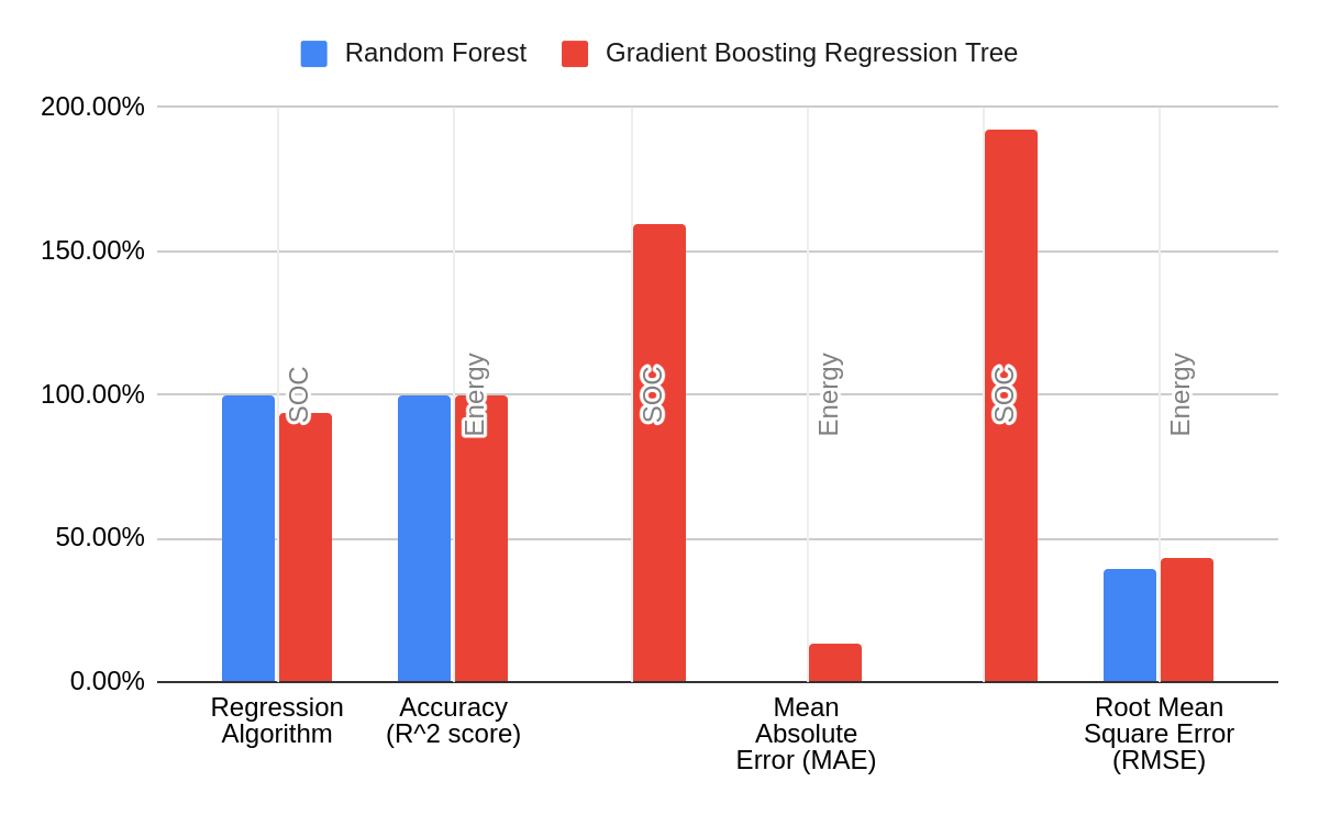
Comparison:

By comparing the accuracies of the two models, RF and GBRT, we see that the RF algorithm performs better than the other over the same training set. While GBRT gives a comparable accuracy as that of RF in predicting the energy, the main difference comes in predicting the SOC.

So the RF model would be a better choice for data estimation, as seen from the experiments performed on the data generated from the MATLAB simulations.

Regression Algorithm	Accuracy (R^2 score)		Mean Absolute Error (MAE)		Root Mean Square Error (RMSE)
	SOC	Energy	SOC	Energy	SOC	Energy
Random Forest	99.9%	99.9%	0.0007	0.0042	0.0008	0.3944
Gradient Boosting Regression Tree	93.5%	99.9%	1.5948	0.1324	1.9202	0.4312

Conclusion

The development of an efficient battery management system using the previously-mentioned methods would help build safer EVs. By making data analysis more practical, the research being conducted would help reduce the gap between the tests in labs and the real-time conditions. This will help prevent any accidents that can be caused by faults in batteries.

The data generated from the MATLAB simulations were extracted and the essential parameters served as the input to the two different machine learning algorithms used to predict the SOC and power/energy consumed. Promising results were obtained with more than 90% accuracy in the regression models, and I believe that this can be increased with the help of more data.