
Assignment 1: Rendering Basics with PyTorch3D
Questions: Github Assignment 1
1. Practicing with Cameras
1.1 360-degree Renders
Usage:
1
python -m submissions.src.render_360 --num_frames 100 --fps 15 --output_file submissions/360-render.gif
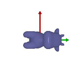
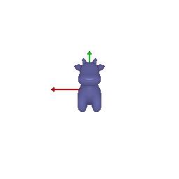
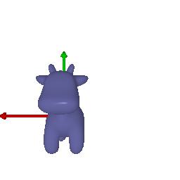
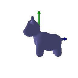
360-degree gif video that shows many continuous views of the provided cow mesh:
1.2 Re-creating the Dolly Zoom
Usage:
1
python -m starter.dolly_zoom --num_frames 20 --output_file submissions/dolly.gif
My recreated Dolly Zoom effect:
2. Practicing with Meshes
2.1 Constructing a Tetrahedron
Usage:
1
python -m submissions.src.mesh_practice --shape tetrahedron --num_frames 50 --fps 15 --output_file submissions/tetrahedron.gif --image_size 512
360-degree gif animation of tetrahedron:

Number of vertices = 4
Number of faces = 4
2.2 Constructing a Cube
Usage:
1
python -m submissions.src.mesh_practice --shape cube --num_frames 50 --fps 15 --output_file submissions/cube.gif --image_size 512
360-degree gif animation of cube:
Number of vertices = 8
Number of faces = 12
3. Re-texturing a mesh
Chosen colors:
color1 = [0, 1, 1]
color2 = [1, 1, 0]
Usage:
1
python -m submissions.src.retexturing_mesh --num_frames 50 --fps 15 --output_file submissions/retexture_mesh.gif --image_size 512
Gif of rendered mesh:
4. Camera Transformations
$1)$ Rotate about z-axis by -90 degrees:
$R_{relative} = [[\cos(-\pi/2), -\sin(-\pi/2), 0], [\sin(-\pi/2), \cos(-\pi/2), 0], [0, 0, 1]]$
Use original translation matrix: $T_{relative} = [0, 0, 0]$
$2)$ Keep original rotation matrix: $R_{relative} = [[1, 0, 0], [0, 1, 0], [0, 0, 1]]$
Move along z-axis by 2: $T_{relative} = [0, 0, 2]$
$3)$ Keep original rotation matrix: $R_{relative} = [[1, 0, 0], [0, 1, 0], [0, 0, 1]]$
Move along x-axis by 0.5 and along y-axis by -0.5: $T_{relative} = [0.5, -0.5, 0]$
$4)$ Rotate along y-axis by 90 degrees: $R_{relative} = [[\cos(\pi/2), 0, \sin(\pi/2)], [0, 1, 0], [-\sin(\pi/2), 0, \cos(\pi/2)]]$
Move along x-axis by -3 and along z-axis by 3: $T_{relative} = [-3, 0, 3]$
5. Rendering Generic 3D Representations
5.1 Rendering Point Clouds from RGB-D Images
Usage:
1
python -m submissions.src.pcl_render --image_size 512
Gif of point cloud corresponding to the first image:
Gif of point cloud corresponding to the second image:
Gif of point cloud formed by the union of the first 2 point clouds:

5.2 Parametric Functions
Usage:
1
python -m submissions.src.torus_render --function parametric --image_size 512 --num_samples 500
Parametric equations of Torus:
\[x = (R + r\cos\theta)\cos\phi \\ y = (R + r\cos\theta)\sin\phi \\ z = r\sin\theta\]where \(\theta \in [0,2\pi) \\ \phi \in [0,2\pi)\)
The major radius $R$ is the distance from the center of the tube to the center of the torus and the minor radius $r$ is the radius of the tube
360-degree gif of torus, with visible hole:

Parametric equations of Superquadric Surface:
\[x = a(\cos\theta)^m(\cos\phi)^n \\ y = b(\cos\theta)^m(\sin\phi)^n \\ z = c(\sin\theta)^m\]where \(\theta \in [-\frac{\pi}{2}, \frac{\pi}{2}] \\ \phi \in [0,2\pi)\)
360-degree gif of Superquadric Surface:
5.3 Implicit Surfaces
Usage:
1
python -m submissions.src.torus_render --function implicit --image_size 512
Implicit equation of torus:
\[F(X,Y,Z) = (R - \sqrt{X^2+Y^2})^2 + Z^2 - r^2\]360-degree gif of torus, with visible hole:
Implicit equation of Superquadric Surface:
\[F(X,Y,Z) = \bigg(\bigg(\bigg\rvert\frac{X}{a}\bigg\rvert \bigg)^\frac{2}{n} + \bigg(\bigg\rvert\frac{Y}{b}\bigg\rvert \bigg)^\frac{2}{n} \bigg)^\frac{n}{m} + \bigg(\bigg\rvert\frac{Z}{c}\bigg\rvert \bigg)^\frac{2}{m} - 1\]360-degree gif of Superquadric Surface:
Tradeoffs between rendering as a mesh vs a point cloud:
- Method of Generation:
- Point Clouds: Formed by directly sampling a parametric function.
- Meshes: Built by voxelizing a 3D space, sampling an implicit function, and then extracting surfaces using the Marching Cubes algorithm.
- Rendering Speed:
- Point Clouds: Faster to render since they simply use sampled points without extra processing.
- Meshes: Slower because they need additional steps like voxelization and surface extraction before rendering.
- Accuracy & Visual Quality:
- Point Clouds: More accurate at capturing fine details because each point represents a sampled location. However, they don’t have surfaces, making shading and texturing more difficult.
- Meshes: Can be less accurate due to voxelization, but increasing the resolution can improve precision. They also provide continuous surfaces, which makes them easier to texture and shade.
- Computational Efficiency:
- Point Clouds: Easier to rotate, scale, and modify since they are just a collection of points.
- Meshes: More computationally expensive to modify because updating a mesh requires adjusting vertex positions and their connections.
6. Do Something Fun
Here is a 360 degree view of a cottage and also a dolly zoom view:
Usage:
1
python -m submissions.src.fun --function full --image_size 512 --output_file submissions/cottage_render_360.gif
Usage:
1
python -m submissions.src.fun --function dolly --image_size 512 --output_file submissions/cottage_dolly.gif
(Extra Credit) 7. Sampling Points on Meshes
Assignment 2: Single View to 3D
Questions: Github Assignment 2
0. Setup
Downloaded the shapenet single-class dataset. Unzipped the dataset and set the appropriate path in dataset_location.py.
1. Exploring loss functions
1.1. Fitting a voxel grid
To align a predicted voxel grid with a target shape, I used a binary cross-entropy (BCE) loss function. A 3D voxel grid consists of 0 (empty) and 1 (occupied) values, making this a binary classification problem where we predict occupancy probabilities of each voxel.
Implementation:
1
2
3
4
5
6
7
8
9
10
def voxel_loss(voxel_src,voxel_tgt):
	# voxel_src: b x h x w x d
	# voxel_tgt: b x h x w x d

	voxel_src.unsqueeze(1)
	voxel_tgt.type(dtype=torch.LongTensor)

	loss = torch.nn.functional.binary_cross_entropy(voxel_src, voxel_tgt)

	return loss
Usage:
1
python fit_data.py --type 'vox'
| Ground Truth | Optimized Voxel |
|---|---|
 |  |
I trained the data for 10000 iterations.
1.2. Fitting a point cloud
Usage:
1
python fit_data.py --type 'point'
| Ground Truth | Optimized Point Cloud |
|---|---|
 |  |
1
2
3
4
5
6
7
8
def chamfer_loss(point_cloud_src,point_cloud_tgt):
	# point_cloud_src, point_cloud_src: b x n_points x 3

	p1 = knn_points(point_cloud_src, point_cloud_tgt)
	p2 = knn_points(point_cloud_tgt, point_cloud_src)
	loss_chamfer = torch.mean(torch.sum(p1.dists + p2.dists))

	return loss_chamfer
1.3. Fitting a mesh
Usage:
1
python fit_data.py --type 'mesh'
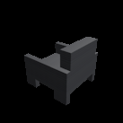
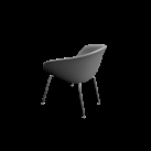
| Ground Truth | Optimized Mesh |
|---|---|
 |  |
1
2
3
4
5
def smoothness_loss(mesh_src):

	loss_laplacian = mesh_laplacian_smoothing(mesh_src)

	return loss_laplacian
2. Reconstructing 3D from single view
2.1. Image to voxel grid
| Input RGB | Ground Truth Mesh | Ground Truth Voxel | Predicted 3D Voxel |
|---|---|---|---|
 |  |  |  |
 |  |  |  |
 |  |  |  |
 |  |  |  |
I implemented the decoder architecture from the paper Pix2Vox: Context-aware 3D Reconstruction from Single and Multi-view Images.
For the encoder, I used the pre-trained ResNet-18 model, which computes a set of features for the decoder to recover the 3D shape of the object.
The decoder is responsible for transforming information of 2D feature maps into 3D volumes. I specifically implemented a slightly modified version of the Pix2Vox-F architecture from the above paper. The input of the decoder is of size [batch_size x 512] and the output is [batch_size x 32 x 32 x 32]. The decoder contains five 3D transposed convolutional layers. The first four transposed convolutional layers are of kernel size $4^3$, with stride of $2$ and padding of $1$. The last layer has a kernel of size $1^3$. Each transposed convolutional layer is followed by a LeakyReLU activation function, except for the last layer which is followed by a sigmoid activation function. The number of output channels for each layer follows the Pix2Vox-F configuration: 128 -> 64 -> 32 -> 8 -> 1.
I trained the model for 10000 iterations, with the default batch size of 32 and learning rate of 4e-4.
Usage:
1
2
3
python train_model.py --type 'vox' --max_iter 10000 --save_freq 500

python eval_model.py --type 'vox' --load_checkpoint
2.2. Image to point cloud
| Input RGB | Ground Truth Mesh | Ground Truth Point Cloud | Predicted 3D Point Cloud |
|---|---|---|---|
 |  |  |  |
 |  |  |  |
 |  |  |  |
 |  |  |  |
I used an approach similar to the Pix2Vox-F decoder that I implemented above. The ResNet-18 model encodes the input images into feature maps, and a decoder reconstructs the 3D shape of the object from them.
The decoder takes in an input of size [batch_size x 512] and gives an output of size [batch_size x n_points x 3]. The decoder architecture comprises of 4 fully connected layers, three of which are followed by a LeakyReLU activation function.
I trained the model for 2000 iterations, with the default batch size of 32 and learning rate of 4e-4.
Usage:
1
2
3
python train_model.py --type 'point' --max_iter 2000 --save_freq 500 --n_points 5000

python eval_model.py --type 'point' --load_checkpoint --n_points 5000
2.3. Image to mesh
| Input RGB | Ground Truth Mesh | Predicted Mesh |
|---|---|---|
 |  |  |
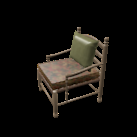 |  |  |
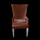 |  |  |
 |  |  |
Instead of encoding an image like I did in case of image to voxel and image to point cloud, the meshes are constructed from an icosphere mesh. The purpose of the decoder is to refine this initial mesh by giving per-vertex displacement vector as an ouput.
The decoder architecture that I implemented is very similar to that in case of image to point cloud, as mentioned above. It takes an input of size [batch_size x 512] and gives an output of size [batch_size x num_vertices x 3]. It comprises of 4 fully connected layers, three of which are followed by a ReLU activation function.
I trained the model for 2000 iterations, with the default batch size of 32, learning rate of 4e-4.
Usage:
1
2
3
python train_model.py --type 'mesh' --max_iter 2000 --save_freq 500

python eval_model.py --type 'mesh' --load_checkpoint
2.4. Quantitative comparisions
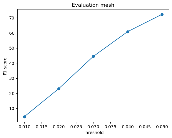
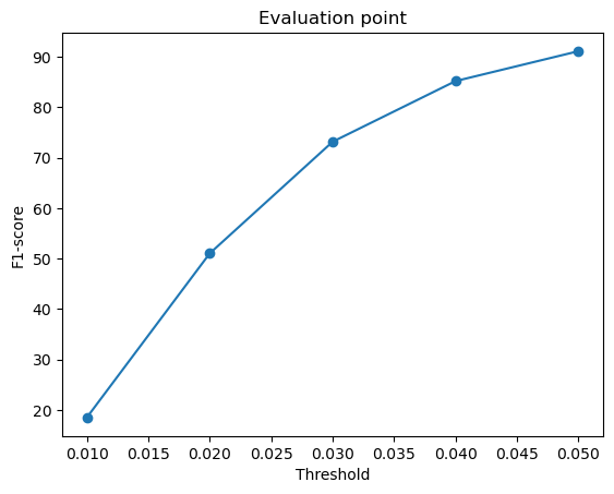
F1-score curves at different thresholds:
| Voxel Grid | Point Cloud | Mesh |
|---|---|---|
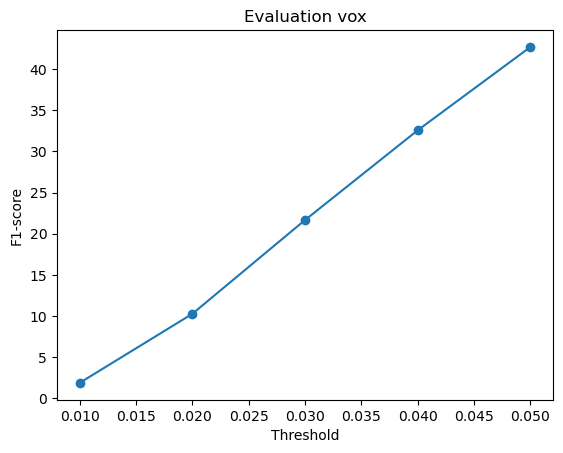 | 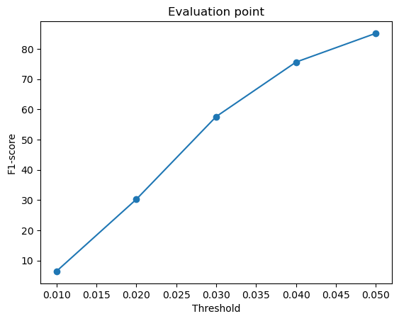 | 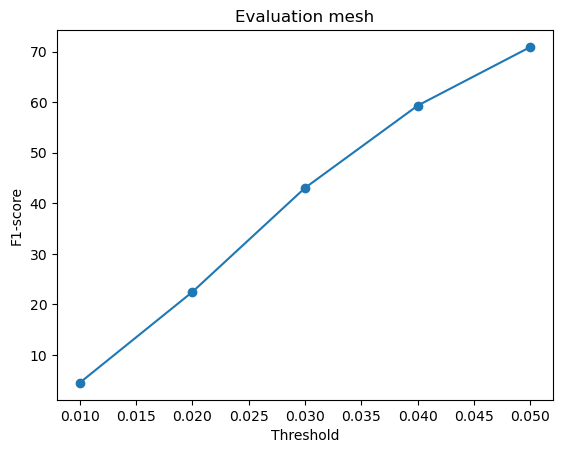 |
From the above plots, we can infer that the point cloud model performed the best, giving the highest F1-score, followed by the mesh model and the voxel model.
Intuitively, I think the reason the point cloud outperformed the voxel and mesh models is because it aligns well with the evaluation method, which compares points directly from the network output to the ground truth. Since point clouds don’t need to define surfaces or connections, they are more flexible and avoid errors caused by surface sampling. This makes them easier to optimize and more accurate in reconstruction.
The mesh model performed slightly worse primarily due to the challenges associated with sampling points from a continuous surface. Unlike point clouds, where each output point is directly predicted, meshes require proper face orientation and connectivity. Due to this, the sampled points might not always align perfectly with the ground truth, especially when dealing with complex geometries like thin structures (legs of the chair).
The voxel model has the lowest F1-score because representing 3D space as voxels limits a lot of detail and accuracy. Fine details can be lost due to this fixed resolution and sampled points may not always align perfectly with the object’s actual surface, affecting evaluation results.
2.5. Analyse effects of hyperparams variations
I have chosen to vary the w_smooth hyperparameter and analyze the changes in the mesh model prediction. The default value of w_smooth is 0.1, and its results have been shown in Section 2.3. I sampled 4 other values of w_smooth - 0.001, 0.01, 1, 10.
| Input RGB | Ground Truth Mesh | w_smooth=0.001 | w_smooth=0.01 | w_smooth=0.1 (Default) | w_smooth=1 | w_smooth=10 |
|---|---|---|---|---|---|---|
 |  |  |  | |  |  |
 |  |  |  | |  |  |
 |  |  |  | |  |  |
F1-score curves for different variations in w_smooth for the mesh model:
w_smooth=0.001 | w_smooth=0.01 | w_smooth=0.1 (Default) | w_smooth=1 | w_smooth=10 |
|---|---|---|---|---|
Avg F1-score@0.05 = 72.977 | Avg F1-score@0.05 = 72.133 | Avg F1-score@0.05 = 70.951 (Default) | Avg F1-score@0.05 = 71.834 | Avg F1-score@0.05 = 72.337 |
 |  | |  |  |
For low values of w_smooth = 0.001, 0.01:
- They preserve the fine details but introduce noise and distortions
- It results in rough and fragmented surfaces
- They show a slightly higher F1-score because they retain geometric details
For high values of w_smooth = 1, 10:
- They produce cleaner and more smooth meshes with reduced artifacts
- It over-smooths the surface, causing loss of sharp details
- The F1-score improves slightly likely because they more likely fall within the threshold radius of the ground truth
The default value of w_smooth = 0.1 falls in between the above two categories.
2.6. Interpret your model
Per-Point Error Visualization
| Input RGB | Ground Truth Point Cloud | Predicted 3D Point Cloud | Per-Point Error |
|---|---|---|---|
| | |  |
| | |  |
I used per-point error to gauge how well each predicted 3D point matches its corresponding point in the ground truth. In my approach, I compute the distance between each point in my reconstructed point cloud and its nearest neighbor in the ground truth. Then, I color-code these distances such that points with very small errors appear in cool colors (blue), while those with larger errors show up in warm colors (red).
From the above gifs, we can clearly see that some regions are rendered in cool tones, which tells me that my model is accurately capturing those parts of the object, such as the seat surface or the main body of the chair. On the other hand, areas highlighted in warm colors reveal where the model struggles, like along the thin chair legs or at complex curves of the backrest.
This visualization pinpoints the exact regions that need improvement.
Failure Case Analysis
In analyzing my 3D voxel model’s predictions, I noticed that while it reconstructs the backrest of chairs quite well, it struggles significantly with legs, seats, and unusual shapes. These failure cases provide valuable insight into the model’s learning behavior and what its limitations are.
Legs: Chair legs vary widely in shape, thickness, and placement across different samples in the dataset. Some chairs have four standard legs, while others may have a single central support or a complex curved base. Because the model tries to generalize patterns across the dataset, it struggles to reconstruct legs consistently. Additionally, legs are usually thin and small compared to the rest of the chair, and this makes them more prone to voxelization errors.
Seats: Many chair designs have gaps in them, which makes it challenging for the model to learn and also more prone to voxelization errors. Since the model tries to reconstruct a smoothed version of objects, it often fails to represent holes correctly, either closing them off entirely or introducing unexpected artifacts.
Unusual shapes: Some chairs in the dataset have very unique designs. Since the model is trained on a limited dataset, it may not have seen enough similar examples to generalize well.
3. Exploring other architectures / datasets
3.3 Extended dataset for training
dataset_location.py updated to include the extended dataset containing three classes (chair, car, and plane).
| category | #instances |
|---|---|
| airplane | 36400 |
| car | 31460 |
| chair | 61000 |
| total | 128860 |
I trained and evaluated the point cloud model with n_points = 5000.
Quantitative evaluation:
| Point Cloud trained on one class | Point Cloud trained on three classes |
|---|---|
|  |
Qualitative evlautaion by comparing “training on one class” vs “training on three classes”:
| Input RGB | Ground Truth Point Cloud | Predicted 3D Point Cloud for 1 Class Training | Predicted 3D Point Cloud for 3 Classes Training |
|---|---|---|---|
 |  |  |  |
 |  |  |  |
 |  |  |  |
3D consistency and diversity of output samples:
Training the model on a single class, like chairs, results in more consistent and refined reconstructions. Since the model only sees one object type during training, it gets really good at capturing the details and structure unique to that class. However, this also means that the model becomes highly specialized. So when it is faced with a completely new object type (such as an airplane or car), it struggles because it hasn’t learned to handle the variation.
On the other hand, training on multiple classes (airplanes, cars, and chairs) allows the model to adapt better to different object shapes. Instead of focusing on one type, it learns general patterns that apply across different categories. This makes it more versatile when reconstructing new objects.
So in conclusion, single-class models tend to produce more uniform outputs because they have learned a very specific structural representation but lack adaptability. Multi-class models generate more diverse outputs because they have seen various object types and have learned to adapt to different shapes but at the cost of some fine-grained details.
Assignment 3: Part-1 Neural Volume Rendering
Questions: Github Assignment 3
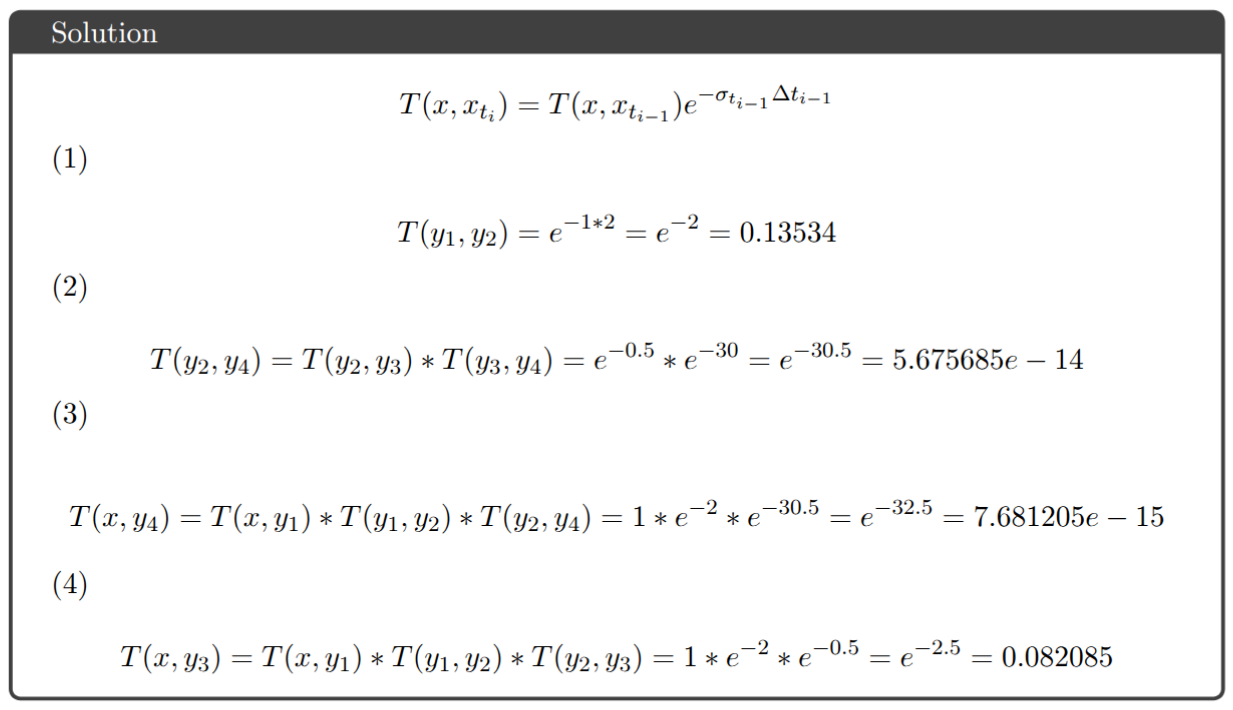
0. Transmittance Calculation
1. Differentiable Volume Rendering
1.3. Ray sampling
Usage:
1
python volume_rendering_main.py --config-name=box
1.4. Point sampling
Usage:
1
python volume_rendering_main.py --config-name=box
1.5. Volume rendering
Usage:
1
python volume_rendering_main.py --config-name=box
2. Optimizing a basic implicit volume
2.1. Random ray sampling
1
2
3
4
5
6
7
def get_random_pixels_from_image(n_pixels, image_size, camera):
    xy_grid = get_pixels_from_image(image_size, camera)

    # Random subsampling of pixel coordinaters
    xy_grid_sub = xy_grid[np.random.choice(xy_grid.shape[0], n_pixels)].to("cuda")

    return xy_grid_sub.reshape(-1, 2)[:n_pixels]
2.2. Loss and training
loss = torch.nn.functional.mse_loss(rgb_gt, out['feature'])
Usage:
1
python volume_rendering_main.py --config-name=train_box
Box center: (0.2502, 0.2506, -0.0005)
Box side lengths: (2.0051, 1.5036, 1.5034)
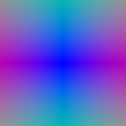
2.3. Visualization
Usage:
1
python volume_rendering_main.py --config-name=train_box
3. Optimizing a Neural Radiance Field (NeRF)
Usage:
1
python volume_rendering_main.py --config-name=nerf_lego
4. NeRF Extras
4.1 View Dependence
Usage:
1
python volume_rendering_main.py --config-name=nerf_materials
Trade-offs between increased view dependence and generalization quality:
- Adding view dependence allows the model to capture complex lighting effects like reflections, and translucency. But excessive view dependence can create inconsistencies when interpolating between unique views, which will make the rendering look unnatural.
- If the network heavily relies on viewing direction, it may overfit to the specific camera angles in the training data. This can lead to poor generalization to unseen viewpoints.
- It can increase the network’s complexity, requiring more parameters and training time.
Assignment 3: Part-2 Neural Surface Rendering
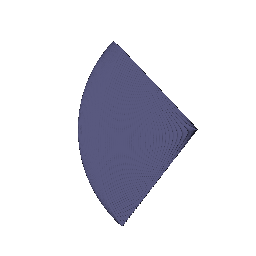
5. Sphere Tracing
My implementation of the SphereTracingRenderer class uses the sphere tracing algorithm to find intersections between rays and an implicit surface of a torus defined by a signed distance field. The algorithm iteratively updates points along each ray by moving in the direction of the ray by the amount of the SDF value at the current point. This process continues until the maximum number of iterations is reached or the SDF value becomes very close to zero (threshold of 1e-6), indicating a surface intersection.
Usage:
1
python -m surface_rendering_main --config-name=torus_surface
6. Optimizing a Neural SDF
Usage:
1
python -m surface_rendering_main --config-name=points_surface
| Input | lr=0.0001 | lr=0.001 | lr=0.00001 |
|---|---|---|---|
 |  |  |  |
| Loss | 0.001279 | 0.000428 | 0.001635 |
eikonal_loss = ((gradients.norm(2, dim=1) - 1.0) ** 2).mean()
Implementation:
1
2
3
4
5
6
Input (XYZ points) -> Harmonic Embedding -> Layer 1 (Linear + ReLU)
                      -> Layer 2 (Linear + ReLU)
                      -> Layer 3 (Linear + ReLU)
                      -> ...
                      -> Layer N (Linear + ReLU)
                      -> Linear SDF (Output: Signed Distance Function)
7. VolSDF
Usage:
1
python -m surface_rendering_main --config-name=volsdf_surface
- Alpha: Scales the overall density. A higher value increases the density, while a lower value reduces it.
- Beta: Controls how quickly the density changes with distance from the surface. A smaller beta results in a sharper transition, while a larger beta smooths the transition.
1
2
3
4
5
6
def sdf_to_density(signed_distance, alpha, beta):
    return torch.where(
            signed_distance > 0,
            0.5 * torch.exp(-signed_distance / beta),
            1 - 0.5 * torch.exp(signed_distance / beta),
        ) * alpha
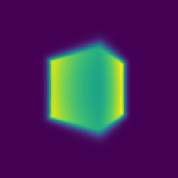
| Geometry | Result |
|---|---|
 |  |
| Loss | 0.006958 |
The above renders are for values alpha=10.0 and beta=0.05.
When alpha=10.0 and beta is changed:
beta | beta=0.05 | beta=0.1 | beta=0.5 |
|---|---|---|---|
| Geometry | |  |  |
| Render | |  |  |
| Loss | 0.006958 | 0.010227 | 0.020789 |
When beta=0.05 and alpha is changed:
alpha | alpha=1 | alpha=10 | alpha=50 |
|---|---|---|---|
| Geometry |  | |  |
| Render |  | |  |
| Loss | 0.022317 | 0.006958 | 0.004329 |
How does high beta bias your learned SDF? What about low beta?
High beta makes the transition between occupied and free space more gradual, leading to a smoother SDF. This can cause a bias where surfaces appear more diffused rather than sharp.
Low beta results in a sharper transition, meaning the SDF will be more precise in distinguishing surfaces, but it can also lead to unstable gradients and more difficult optimization.
Would an SDF be easier to train with volume rendering and low beta or high beta? Why?
An SDF is generally easier to train with volume rendering when using a high beta. This is because high beta values cause a larger number of points along each ray to have non-zero density, allowing gradients to be backpropagated through more points simultaneously. This leads to denser gradients and faster convergence during training.
Training with a low beta can be more challenging because it forces the network to learn very sharp transitions, which means only points very close to the surface contributes significantly to the rendering. This can lead to sparse gradients and slower convergence.
Would you be more likely to learn an accurate surface with high beta or low beta? Why?
You are more likely to learn an accurate surface with a low beta. A low beta encourages sharp boundaries and a more precise surface representation, as the density function closely approximates a step function. High beta values, on the other hand, lead to smoother surfaces, which can be less accurate.
Implementation:
1
2
3
4
5
6
Input (SDF Feature + XYZ Embedding) -> Layer 1 (Linear + ReLU)
                      -> Layer 2 (Linear + ReLU)
                      -> Layer 3 (Linear + ReLU)
                      -> ...
                      -> Layer N (Linear + ReLU)
                      -> Linear RGB (Output: 3D Color Prediction)
8. Neural Surface Extras
8.3 Alternate SDF to Density Conversions
Logistic density distribution function:
\[\phi_s(x) = \frac{se^{-sx}}{(1+e^{-sx})^2}\]1
2
def neus_sdf_to_density(signed_distance, s):
return s * torch.exp(-s * signed_distance) / ((1 + torch.exp(-s * signed_distance))**2)
s | s=10 | s=50 |
|---|---|---|
| Geometry |  |  |
| Render |  |  |
| Loss | 0.005590 | 0.006529 |
Low s results in a more blurry render, while a higher value of s makes it look sharp.
Assignment 4
Questions: Github Assignment 4
1. 3D Gaussian Splatting
1.1 3D Gaussian Rasterization
Run:
1
python render.py --gaussians_per_splat 1024
Output GIF:
1.2 Training 3D Gaussian Representations
Run:
1
python train.py --gaussians_per_splat 2048 --device cuda
I modified the run_training function to improve performance and reduce CUDA memory usage. Specifically, I:
Reduced the number of Gaussians from 10k to 7k by subsampling the points file, lowering the overall GPU memory footprint.
Ensured key Gaussian parameters (opacities, scales, colours, and means) were trainable and set up an optimizer with different learning rates for each parameter group (as mentioned in 1.2.1)
Wrapped the forward pass in
autocastand usedGradScalerto scale the loss, which both reduced memory usage and accelerated computation
I called the scene.render method to generate the predicted image from the input camera parameters, using the specified image size, background color, and the number of Gaussians per splat. I then computed the L1 loss between the rendered (predicted) image and the ground truth image.
Learning rates that I used for each parameter:
pre_act_opacities=0.001pre_act_scales=0.001colours=0.02means=0.0002
Number of iterations that I trained the model for = 1000
Mean PSNR: 27.356
Mean SSIM: 0.915
Training final render GIF:
Training progress GIF:
1.3 Extensions
1.3.1 Rendering Using Spherical Harmonics
Run:
1
python render.py --gaussians_per_splat 1024
GIF:
| Original | Spherical Harmonics |
|---|---|
|  |
RGB image comparisons of the renderings obtained from both the cases:
| Frame | Original | Spherical Harmonics |
|---|---|---|
| 000 |  | 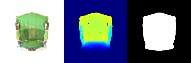 |
| 015 | 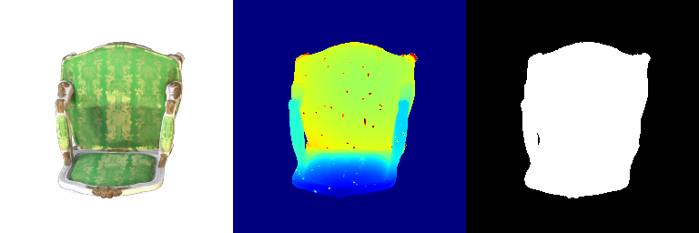 |  |
| 021 | 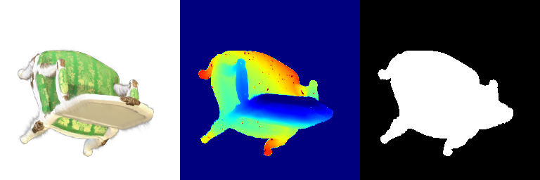 | 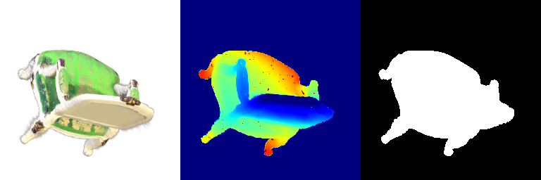 |
| 030 | 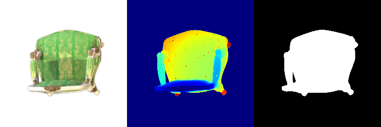 | 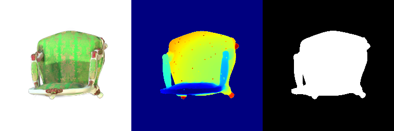 |
Differences that can be observed:
- Frame 000 and 015: The spherical harmonics rendering looks more photorealistic because the angular variations in color better capture how the material responds to illumination from different directions.
- Frames 021 and 030: The spherical harmonics rendering looks more glossy and reflective because the added directional sensitivity leads to more dynamic and detailed shading.
2. Diffusion-guided Optimization
2.1 SDS Loss + Image Optimization
Run:
1
python Q21_image_optimization.py --sds_guidance 1
| Prompt | Without Guidance | With Guidance |
|---|---|---|
| Iterations | 400 | 2000 |
| “a hamburger” |  | 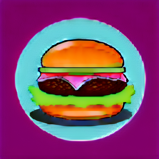 |
| “a standing corgi dog” |  | 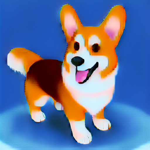 |
| “a fish in a pan” |  | 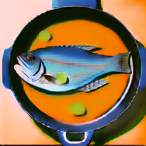 |
| “a mansion” |  | 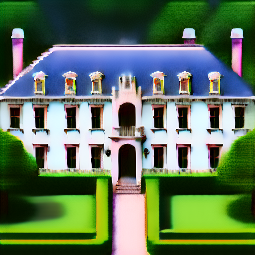 |
2.2 Texture Map Optimization for Mesh
Run:
1
python python Q22_mesh_optimization.py
In order to reduce the CUDA memory footprint, I reduced the image size to 256x256.
| Prompt | Initial Mesh GIF | Final Mesh GIF |
|---|---|---|
| “a tiger” |  |  |
| “a zebra” |  |  |
2.3 NeRF Optimization
I perfomed no CUDA memory optimization here. All values were the same as default as pulled from GitHub.
Prompt: “a standing corgi dog”
Run:
1
python Q23_nerf_optimization.py --prompt "a standing corgi dog" --lambda_entropy 1e-2 --lambda_orient 1e-2 --latent_iter_ratio 0.1
Rendered RGB video:
Rendered depth video:
Prompt: “a hamburger”
Run:
1
python Q23_nerf_optimization.py --prompt "a hamburger" --iters 2500 --lambda_entropy 1e-3 --lambda_orient 1e-2 --latent_iter_ratio 0.2
Rendered RGB video:
Rendered depth video:
Prompt: “a mansion”
Run:
1
python Q23_nerf_optimization.py --prompt "a mansion" --iters 2500 --lambda_entropy 1e-2 --lambda_orient 1e-2 --latent_iter_ratio 0.1
Rendered RGB video:
Rendered depth video:
2.4 Extensions
2.4.1 View-dependent text embedding
Prompt: “a standing corgi dog”
Run:
1
python Q23_nerf_optimization.py --prompt "a standing corgi dog" --lambda_entropy 1e-2 --lambda_orient 1e-2 --latent_iter_ratio 0.1 --view_dep_text 1
Rendered RGB video:
Rendered depth video:
Prompt: “a hamburger”
Run:
1
python Q23_nerf_optimization.py --prompt "a hamburger" --iters 2500 --lambda_entropy 1e-3 --lambda_orient 1e-2 --latent_iter_ratio 0.2 --view_dep_text 1
Rendered RGB video:
Rendered depth video:
Comparing with 2.3:
In 2.3, the NeRF model used one fixed text embedding for all views. This led to consistent but somewhat flat results and sometimes produced artifacts like multiple front faces (standing corgi dog example) because the model didn’t know how to adjust for different angles.
With view-dependent text conditioning, different embeddings (like front, side, and back) are used based on the camera angle. This helps the model adjust lighting, highlights, and reflections for each view, resulting in more realistic and 3D-consistent images.
The “hamburger” looks really good with view-dependent conditioning, while the “standing corgi dog” did not turn out as well, likely because it needs more training to capture all its details.
Assignment 5
Questions: Github Assignment 5
1. Classification Model
Run:
1
2
3
python train.py --task cls

python eval_cls.py
The model was trained for 250 epochs, and the best model was saved at epoch 115.
Train loss = 1.1288
Test accuracy of best model = 0.9696
Visualization of a few random test point clouds and their predicted classes:
| Correct Prediction | Chairs | Vases | Lamps |
|---|---|---|---|
| Point Cloud |  |  |  |
| Point Cloud |  |  |  |
Visualization of a failure prediction for each class:
| Correct Label | Vase | Lamp | Vase |
|---|---|---|---|
| Point Cloud |  |  |  |
| Incorrect Prediction | Lamp | Vase | Lamp |
The successful results show that the model is able to pick out important features. For example, it correctly identifies the distinct structure of chairs, vases, and lamps. But in some cases, the shapes can be ambiguous or similar, which causes the model to misclassify objects. This can happen when the point sampling misses some important details or when the features are too similar between classes.
2. Segmentation Model
Run:
1
2
3
python train.py --task seg

python eval_seg.py
The model was trained for 250 epochs, and the best model was saved at epoch 225.
Train loss = 13.0442
Test accuracy of best model = 0.8966
Visualization of correct segmentation predictions along with their corresponding ground truth:
| Accuracy | 0.9317 | 0.9147 | 0.9308 |
|---|---|---|---|
| Ground Truth |  |  |  |
| Good Segmentation Predictions |  |  |  |
Visualization of incorrect segmentation predictions along with their corresponding ground truth:
| Accuracy | 0.5604 | 0.5572 | 0.4702 |
|---|---|---|---|
| Ground Truth |  |  |  |
| Bad Segmentation Predictions |  |  |  |
The good segmentation predictions show that the model can distinguish the chair’s seat, back, and legs fairly accurately. In the failure cases, we can see that certain parts like the seat or back merges with the legs or other regions. A possible reason could be that if the training data includes ambiguous or poorly differentiated boundaries, the model may struggle to learn to differentiate segments in these areas.
3. Robustness Analysis
3.1 Rotate Input Point Clouds
3.1.1 Classification Model
Visualization of a few random test point clouds and their predicted classes:
| Angle | Accuracy | Chairs | Vases | Lamps |
|---|---|---|---|---|
| 10 degrees | 0.958 | Successful | Successful  | Successful  |
| 10 degrees | 0.958 | Successful  | Successful  | Successful  |
| 20 degrees | 0.894 | Successful | Successful  | Successful  |
| 20 degrees | 0.894 | Wrong predicted as lamp  | Successful  | Successful  |
| 30 degrees | 0.679 | Successful | Successful  | Successful  |
| 30 degrees | 0.679 | Wrong predicted as lamp  | Wrongly predicted as lamp  | Successful  |
| 60 degrees | 0.299 | Wrongly predicted as vase  | Successful  | Wrongly predicted as chair  |
| 60 degrees | 0.299 | Wrong predicted as lamp  | Wrongly predicted as lamp  | Successful  |
From the observations above, we see that the model classifies most rotated objects correctly when the rotation is small (10 or 20 degrees). However, as the rotation angle becomes larger (30 or 60 degrees), the accuracy drops and the model starts confusing objects. This happens because the model wasn’t trained with any rotational variations and so the learned features become orientation-dependent.
3.1.2 Segmentation Model
| Angle | Model | X | X | X | X |
|---|---|---|---|---|---|
| 10 degrees | Ground Truth |  |  |  |  |
| 10 degrees | Prediction | Success: 0.9185  | Success: 0.9134  | Success: 0.9055  | Failure: 0.4798  |
| 20 degrees | Ground Truth |  |  |  |  |
| 20 degrees | Prediction | Success: 0.9396  | Success: 0.9191  | Success: 0.9307  | Failure: 0.5906  |
| 30 degrees | Ground Truth |  |  |  | |
| 30 degrees | Prediction | Success: 0.9093  | Success: 0.9429  | Failure: 0.4707  | |
| 60 degrees | Ground Truth |  |  |  | |
| 60 degrees | Prediction | Failure: 0.4707  | Failure: 0.5283  | Failure: 0.5478  |
From the observations above, we see that the model segments most portions of the rotated objects well when the rotation is small (10 or 20 degrees). However, as the rotation angle becomes larger (30 or 60 degrees), we see a massive accuracy drop. This happens because the model wasn’t trained with any rotational variations and so the learned features become orientation-dependent. The rotations make it difficult for the network to correctly differentiate between segments.
3.2 Different Number of Point Points per Object
3.2.1 Classification Model
| Number of Points | Accuracy | Chairs | Vases | Lamps |
|---|---|---|---|---|
| 5000 | 0.968 | Successful | Successful  | Successful  |
| 1000 | 0.9695 | Successful | Successful  | Successful  |
| 500 | 0.9622 | Successful | Successful  | Successful  |
| 100 | 0.882 | Successful | Successful  | Successful  |
We see that the classification model performs well even with fewer points. The drop in accuracy when the number of points is reduced to 100 or below is expected because fewer points reduce geometric detail, which makes it harder to distinguish specific features. Still, even at 100 points, the outline structure is preserved, allowing the model to classify successfully in many cases.
3.2.2 Segmentation Model
| Number of Points | Model | X | X | X | X |
|---|---|---|---|---|---|
| 5000 | Ground Truth |  |  |  |  |
| 5000 | Prediction | Success: 0.9448  | Success: 0.992  | Success: 0.9658  | Failure: 0.5366  |
| 1000 | Ground Truth |  |  |  |  |
| 1000 | Prediction | Success: 0.952  | Success: 0.988  | Success: 0.904  | Failure: 0.515  |
| 500 | Ground Truth |  |  |  |  |
| 500 | Prediction | Success: 0.934  | Success: 0.998  | Success: 0.926  | Failure: 0.484  |
| 100 | Ground Truth |  |  |  |  |
| 100 | Prediction | Success: 0.92  | Success: 0.96  | Success: 0.91  | Failure: 0.58  |
We see that the segmentation model performs well even with fewer points. While the model performs well even with 500 points, the performance becomes more unstable at 100 points, especially in complex or ambiguous regions. This is because fewer points reduce the structural detail, making it harder for the model to distinguish fine boundaries and specific object features like thin legs and armrests.
4. Bonus Question - Locality
I implemented a general Transformer framework for both the classification model and the segmentation model.
The classification model predicts a single label for an entire point cloud. Each point’s 3D coordinates are passed through two linear layers: one to embed the input features, and another to learn positional information. These two embeddings are added together and fed into a standard Transformer Encoder. After processing, I apply max pooling across all points to extract a global feature vector. This is then passed through fully connected layers with batch normalization, ReLU activation, and dropout. The log softmax over the class scores is then returned.
The segmentation model /assets/images/L3D/a5/outputs a class label for each point. I embed the 3D points and add positional information before passing them through a Transformer Encoder. Instead of pooling the features, I use 1D convolution layers to generate per-point predictions. These /assets/images/L3D/a5/outputs are also passed through a log softmax to get per-point class probabilities.
4.1 Classification Model using Transformers
Run:
1
2
3
python train.py --task cls

python eval_cls.py --load_checkpoint best_model --/assets/images/L3D/a5/output_dir ".//assets/images/L3D/a5/output/Q4/cls"
The model was trained for 100 epochs, and the best model was saved at epoch 18.
Train loss = 30.6177
Test accuracy of best model = 0.9454
Visualization of a few random test point clouds and their predicted classes using Transformers:
| Correct Prediction | Chairs | Vases | Lamps |
|---|---|---|---|
| Point Cloud |  |  |  |
| Point Cloud |  |  |  |
Visualization of a failure prediction for each class using Transformers:
| Correct Label | Vase | Lamp | Lamp |
|---|---|---|---|
| Point Cloud |  |  |  |
| Incorrect Prediction | Lamp | Vase | Chair |
The model was run only for 100 epochs because it was taking a lot of time. I also did not have the time to run the segmentation Transformer model. However, there were no errors in starting the training and it only had to be left running for ~8 hours on my laptop.
Moreover, the Transformer model gave a very high accuracy of 94% for just training for 100 epochs. The classification model without Transformer gave an accuracy of 97% for training for 250 epochs.