Thruster Control of AUV Using LQR

Abstract

• To make two different control system models in Simulink on PID and LQR controllers respectively and to get the results for positional and velocity parameters of the ROV based on the desired reference inputs.
• To tune parameters related to both the controllers to achieve better results and finally test the model physically underwater.

PID Controller

Literature Review

The basic mathematical model of an ROV is given by:

\[\dot{\eta}=J(\eta)v \newline M\dot{v}+C(v)v + D(v)v + g(\eta)=\tau\]

• where M = Mass matrix (with added mass effect taken into account)
• C = Coriolis force matrix
• D = Damping forces matrix
• g = Restoring forces matrix
• $\tau$ = Forces & moments matrix

1. Added Mass Effect:

The added mass of an object is the effect in which some mass of fluid surrounding the object under observation is accelerated/decelerated along with it.

2. Coriolis Effect:

The Coriolis force is a fictitious force that comes into play whenever we are trying to explain the forces on an object with respect to a rotating frame.

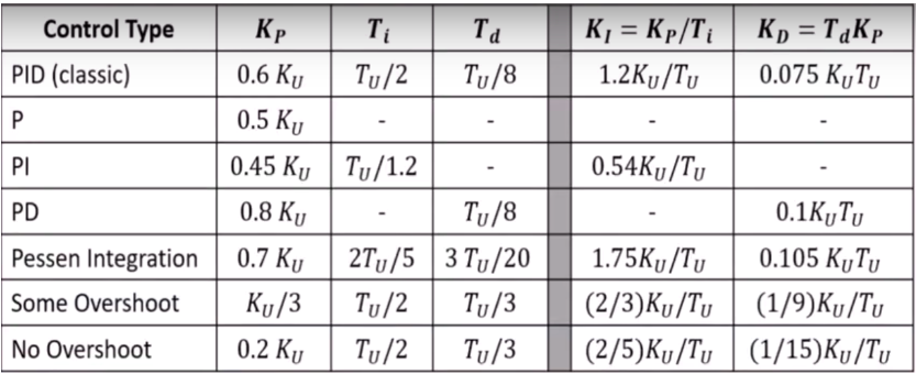
3. Ziegler-Nichols Method for tuning PIDs:

This method can be used to tune our PID both in the case where we have a working model for our plant or even when we don’t. The first step to this method is measuring two parameters: KU which is the gain at which the system becomes marginally stable and TU which is the period of oscillation at marginal system response. These values are found by taking KI and KD values to be zero for that input and changing KP until marginal stability is achieved.

After these parameters are evaluated controller gains can simply be calculated from the below table:

4. Controller Models:

The two controller models that we used are:

1. Linear Model
2. Non-linear Model

Linear Model

The schematic of the simulink model created using the linear PID control looks like this:

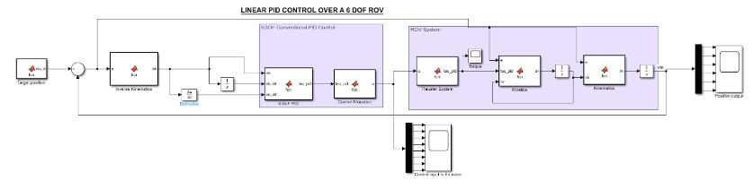
It consists of different functionalities in each block of the design:

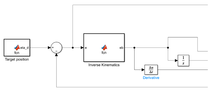
The PID controller uses an error signal, called the tracking error, generated from the difference between the desired position and the current position of the rover.

\[e = \eta_d - \eta\]

This error signal, in the world frame, is converted to the error signal in body frame 𝑒b using the following equation:

\[e^b = J^T(\eta)e\]

where the transformation matrix from the vehicle body frame to the world reference frame using Euler angle transformation is given by:

\[J_\theta(\eta) = \begin{bmatrix} R^n_b(\theta) & 0_{3x3} \\ 0_{3x3}& T_\theta(\theta) \end{bmatrix}\]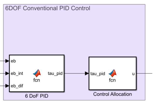

Using the error signal in the body frame 𝑒b, the torque generated by the PID can be calculated using the equation:

\[\tau_{P I D}=K_P e^b(t)+K_I \int_0^t e^b\left(t^{\prime}\right) d t^{\prime}+K_D \frac{d e^b(t)}{d t}\]

In order to generalise the required control forces, control allocation calculates the control input signal u to apply to the thrusters. The control forces due to the control inputs applied to the thrusters can be expressed as:

\[\tau = T(\alpha)F = T(\alpha)Ku\]

As a result, the control input vector can be derived as:

\[u = K^{-1}T^{-1}\tau\]

For the linear model, the following values of KP, KI, and KD have been obtained using the Ziegler-Nichols method:

6-DoF PID	Surge	Sway	Heave	Roll	Pitch	Yaw
KP	3	3	3	4	4	2
KI	0.2	0.2	0.2	0.3	0.3	0.1
KD	2.5	2.5	0.5	0.5	1	0.5

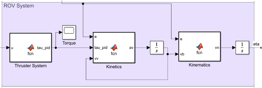
Using the control input vector, the thruster system generates the control forces in 6 DoFs with the help of the above mentioned equation $\tau = T(\alpha)F = T(\alpha)Ku$

Since the 8 thrusters of the ROV produce a maximum thrust of 40N at operating voltage of 16V, the thrust coefficients are approximated to 40. Thus the thrust coefficient matrix 𝐾 is taken as

$K = diag[40,40, 40,40,40,40,40,40]$

After obtaining the torque vector, the kinetics is used to determine the acceleration in the body frame for the given forces using the state equation:

\[M\dot{v}+C(v)v + D(v)v + g(\eta)=\tau\]

The kinematics block is then used to define the vehicle velocity in the world frame 𝑣n. The position of the vehicle is then determined in the integrator and, using inverse kinematics, is converted to the body frame before being supplied back into the controller.

Non-Linear Model

Because of disturbances underwater like current speed, there will be non-linearities introduced into the system. This makes the linear-PID controller model inappropriate to use as there will be a lot of deviations from the desired o/p and noise in the system. So, we need to include the system dynamics to get the control input to the thrusters.

In the nonlinear model-based PID control system design, the dynamic model of the ROV is utilized to produce a 6-DoF predictive force and the model-based PID is used to provide a corrective force in 6 DoFs to adjust the error in the model. This is advantageous in that the model error and non-linearities tend to be smaller than the dynamics themselves.

In the predictive force generation, a virtual reference trajectory strategy is introduced for the design of trajectory tracking. With the use of a scalar measure of tracking in Fossen (Fossen, 1994), a virtual reference $x_r$ can be defined that satisfies:

\[\dot{x_r}=\dot{x_d}+\lambda e^b\]

where $\lambda$ > 0 is the control bandwidth that describes the amount of tracking error to the overall tracking performance, and $e^b$ is the tracking error in the body frame.

Since the velocity $v$ is the time derivative of the position (i.e. $v=\dot{\eta}$), for a defined virtual reference position $\eta_r$, the following is satisfied:

\[v_r=v_d+\lambda e^b\]

So, $\lambda$ is used to tune the 6-DoF predictive force.

This is shown in the following block:

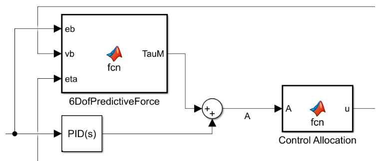
Where ‘A’ is the new controller output.

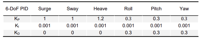
The PID controller gains(Kp, Ki and Kd) for the non-linear model are found out by Ziegler Nichols method and were found out to be as follows:

Finally, the control law for the nonlinear model-based PID controller is computed given by:

\[\begin{aligned}\tau= & M\left(v_d+\lambda\left(v_d-v\right)\right)+C_{R B}(v) v+C_A\left(v_w\right) v_w+D\left(v_w\right)\left(v_d+\lambda e^b-v_c\right)+g(\eta) \\& +K_P e^b(t)+K_I \int_0^t e^b\left(t^{\prime}\right) d t^{\prime}+K_D \frac{d e^b(t)}{d t}\end{aligned}\]

The final model for this system is shown below:

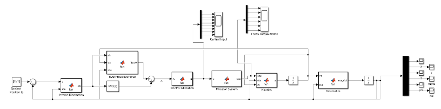
Here, we took desired position input as $[1;1;2;0;0;0]$.

PID Implementation

We implemented the models for both the controllers above and got the following results when we give a desired positional input:

Linear Controller Model

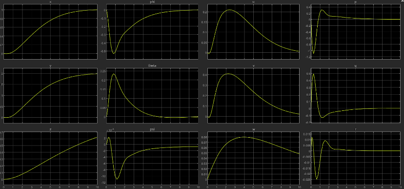
Using the above method, we have obtained the following results for a desired position input: $\eta_d=[3;4;1;1.57;0;0]$.

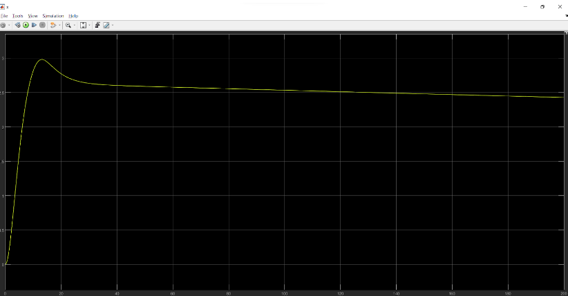
The output of the position and orientation control is obtained as follows:

Position X:

Desired output: 3 m

Obtained result:

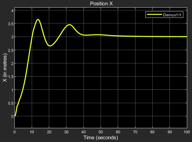
The steady state response final value = 3.

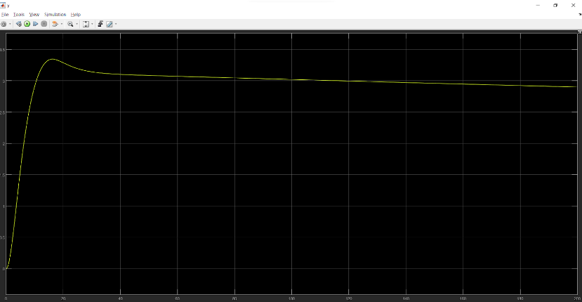
Position Y:

Desired output: 4 m

Obtained result:

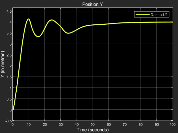
The steady state response final value = 4.

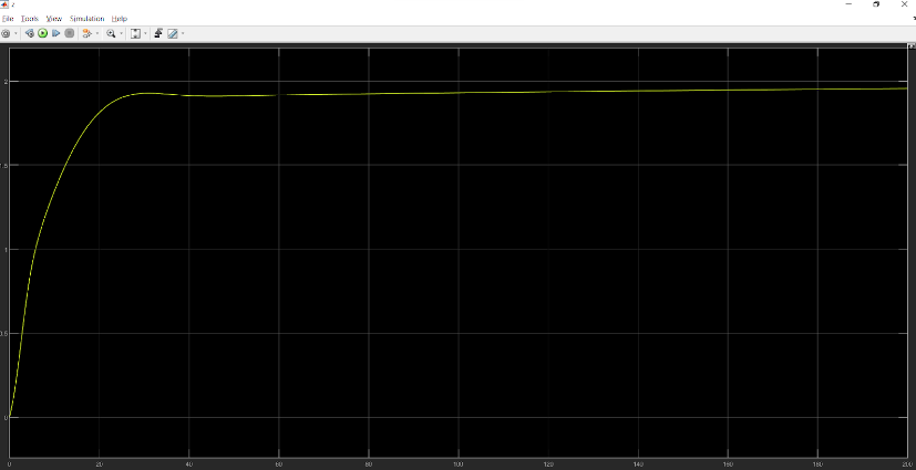
Position Z:

Desired output: 1 m

Obtained result:

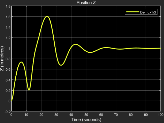
The steady state response final value = 1.

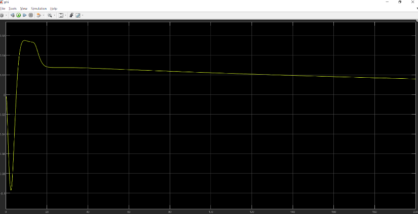
Orientation $\phi$:

Desired output: 1.57 radians

Obtained result:

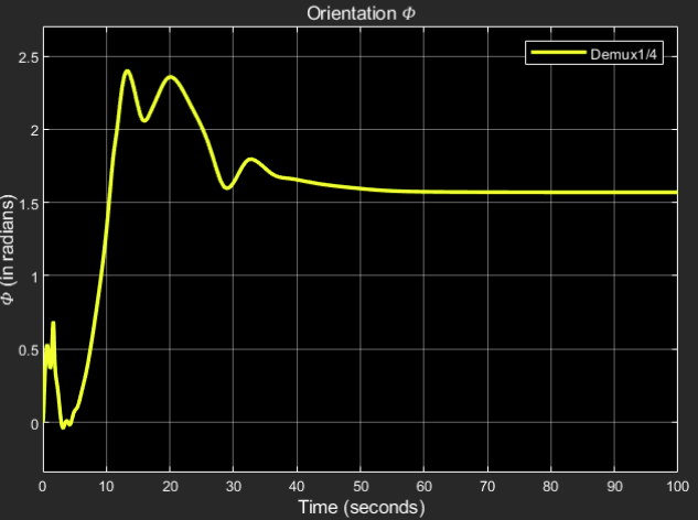
The steady state response final value = 1.57.

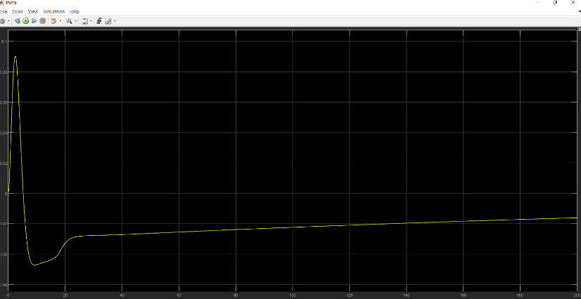
Orientation $\theta$:

Desired output: 0 radians

Obtained result:

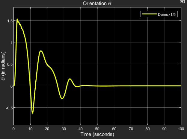
The steady state response final value = 0.

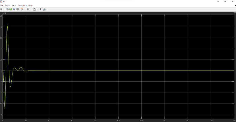
Orientation $\psi$:

Desired output: 0 radians

Obtained result:

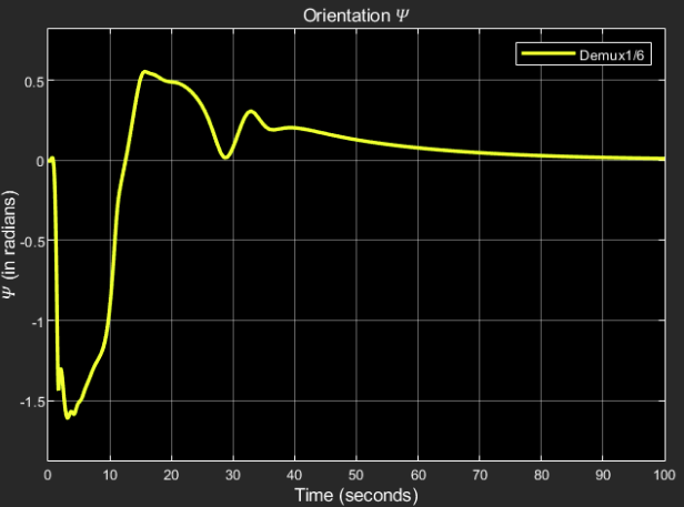
The steady state response final value = 3.

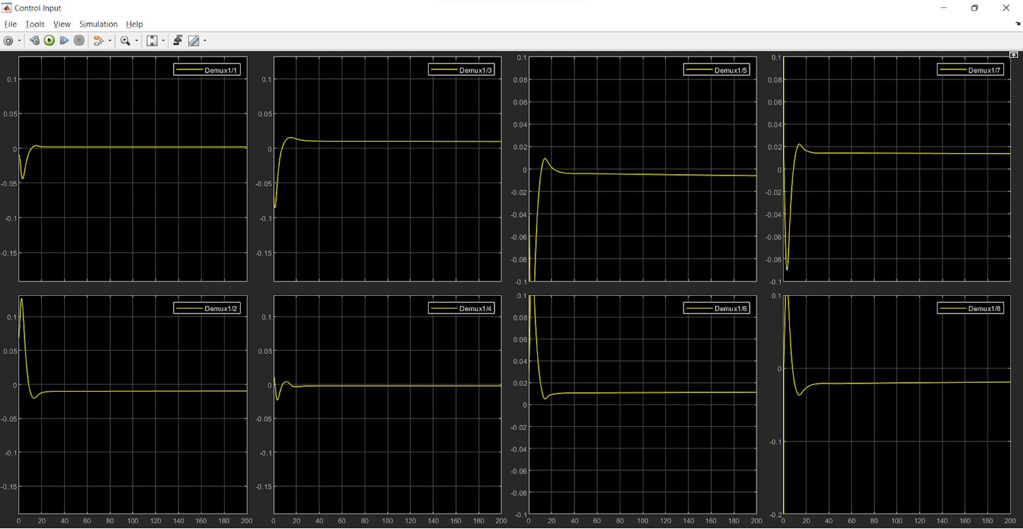
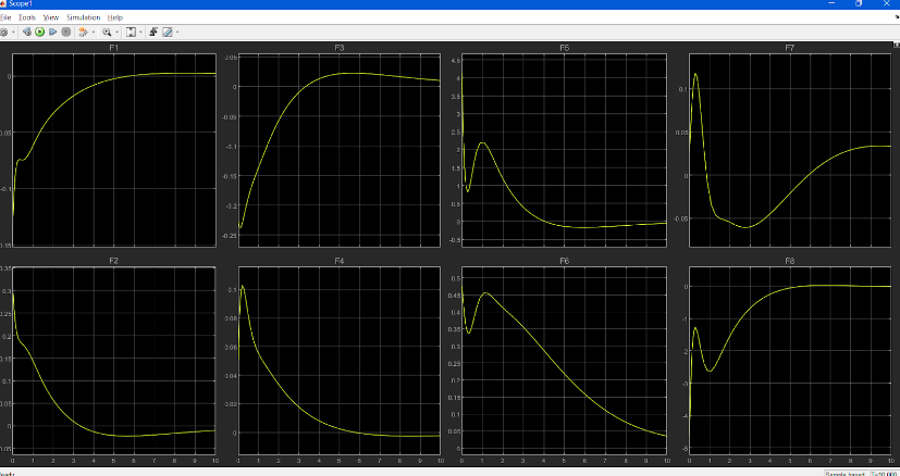
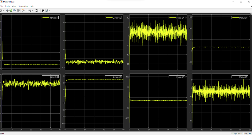
The control inputs to the thrusters for the same are represented in the plots below:

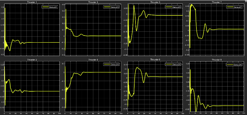
As it is evident from the plots, each thruster is instructed to provide the required thrust every instant for a finite period of time after which the control input eventually settles down to a final value.

The model of the rover under study somewhat looks like this:

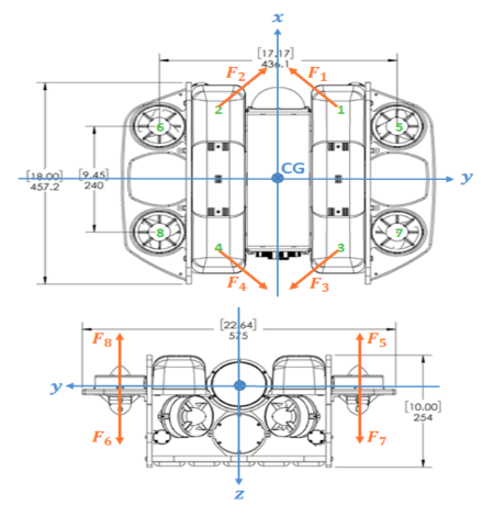
Here, the thrusters 1,2,3,4 are used in the position control in the X,Y directions while 5,6,7,8 are used for the Z-directional control. If we see the plots for the thruster control inputs for 1,2,3,4:

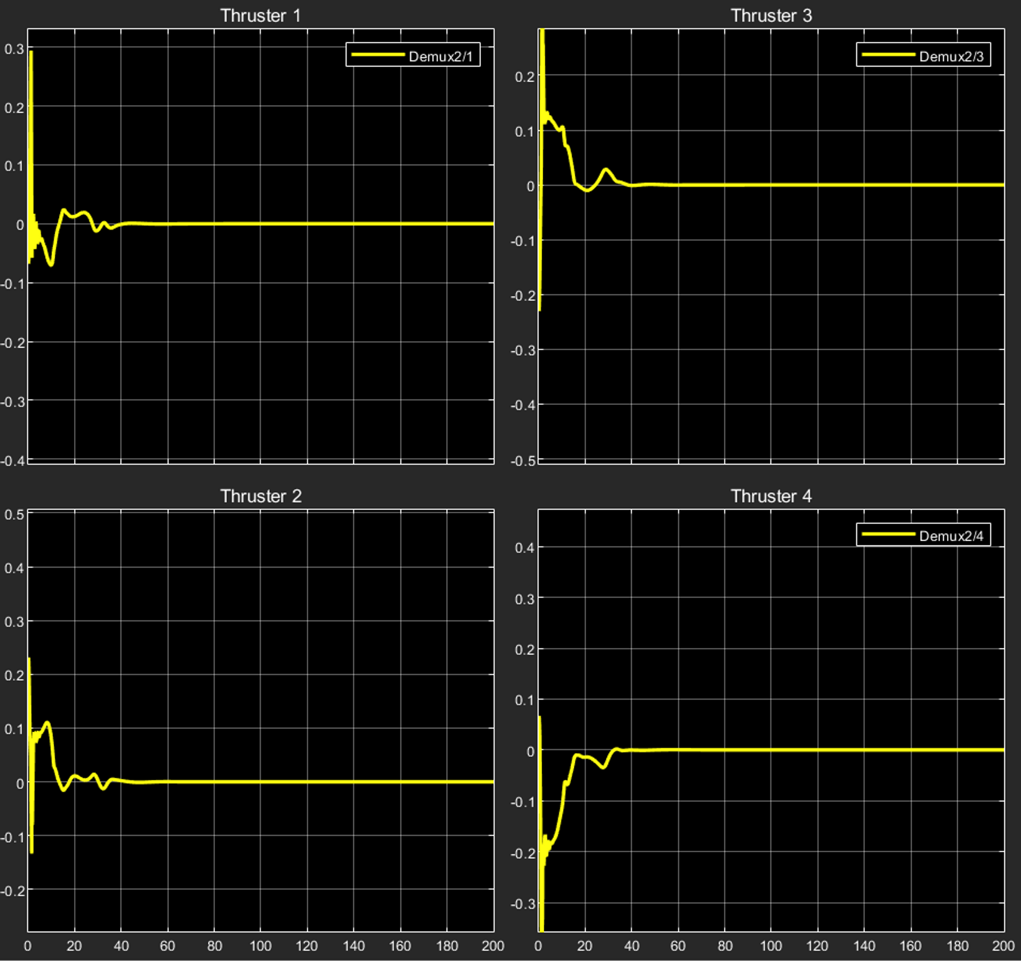
We can observe the steady state final value to be zero for all the thrusters 1,2,3,4.

Reason: The above thrusters are used for controlling the position in X,Y directions and their respective control inputs drive them to work in a synchronised manner so as to reach the respective position. Once the rover has reached the required X,Y, coordinates of the position with the required orientation, there is no need for them to provide any more thrust given the lack of any external force acting in the X,Y directions.

The interesting part comes when we observe the control input plots for the thrusters 5,6,7,8:

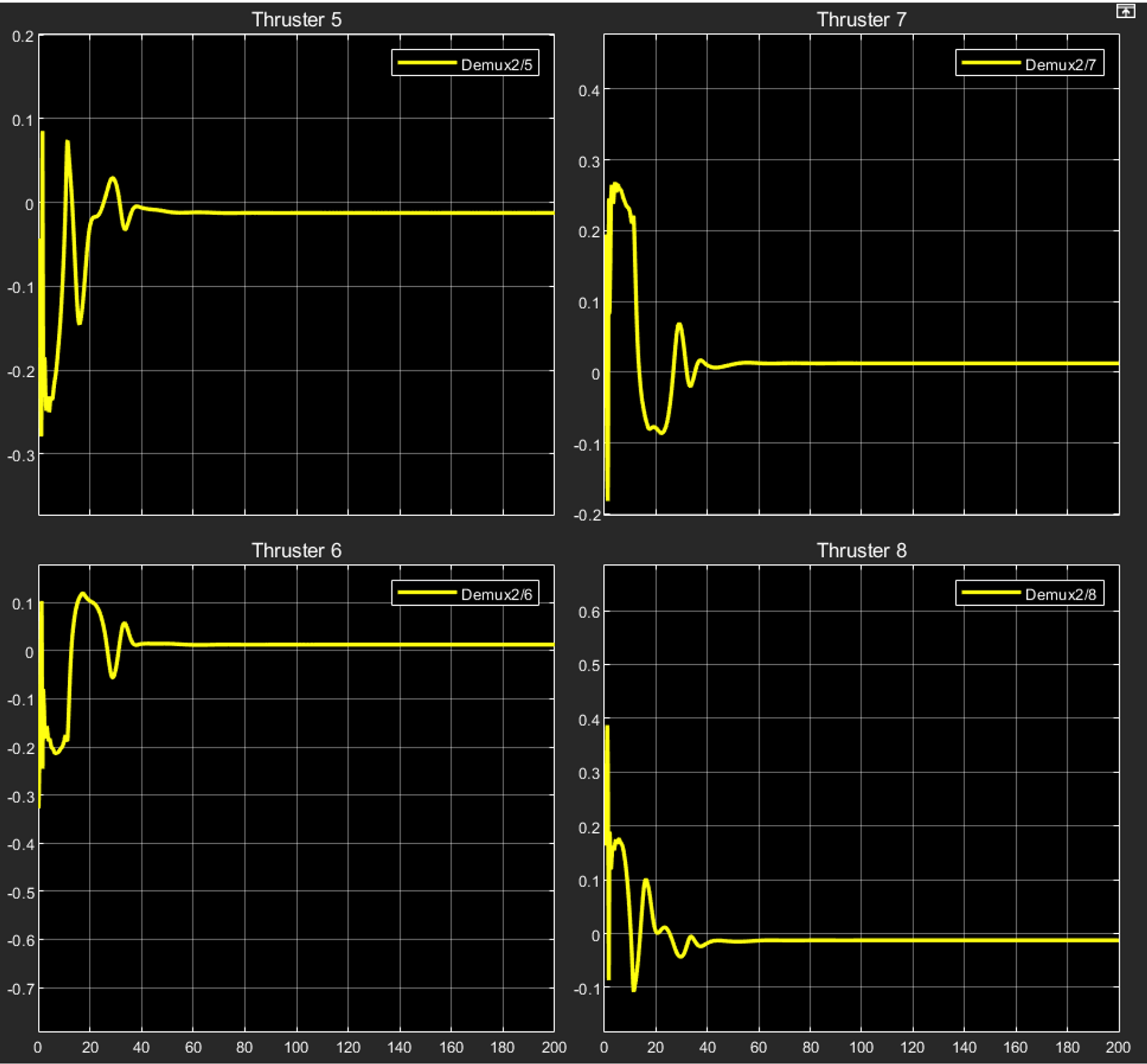
As it is observed, each of the control inputs have a non-zero steady state value; positive for thrusters 6,7 and negative for thrusters 5,8.

Reason: Thrusters 5,6,7,8 are used for positional control in the Z direction. When the rover moves to the desired Z coordinate position in the required orientation, the job of the thrusters is not done since the position has to be retained while neutralising an external force. This external force is the buoyancy acting upon the rover since it is designed to be positively buoyant. The values of forcing acting due to weight and buoyancy for the rover under study are:

W = 112.8 N

B = 114.8 N ; this implies that the net external force acting on the rover is 2N upwards.

When we look at thrusters 5,8 ; they provide a thrust vertically upwards when rotated clockwise while thrusters 6,7 produce a thrust vertically downwards for the same. This means that for thrusters 5,8 positive thrust is upwards while negative thrust is downwards. This is opposite in the case of thrusters 6,7 From the plots of control inputs to the above thrusters, the steady state values are as follows:

For thrusters 5,8: $-1.25*10^{-2}$ (approx.)

For thrusters 6,7: $+1.25*10^{-2}$ (approx.)

Thrust produced by thrusters 5,8 is negative, which implies that thrust is produced in the  vertically downwards direction.

Thrust produced by thrusters 6,7 is positive, which again implies that thrust is produced in the vertically downwards direction.

Total thrust produced $\tau=Ku$ where K= 40 for all the thrusters.

Total thrust produced in steady state:

\[4*1.25*10^{-2}*40=2N\]

downwards.

Since the external force in Z direction has been neutralised, the rover is stabilised once it reaches the desired position.

This is how the positional control of the underwater rover has been established using the linear PID control method.

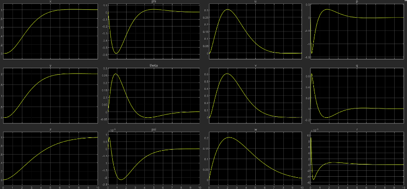
Non-Linear Controller Model

For desired positional input as $[1;1;2;0;0;0]$, we got the following results for positional coordinates in world frame:

Position X:

Desired output: 1 m

Position Y:

Desired output: 1 m

Position Z:

Desired output: 2 m

Orientation $\phi$:

Desired output: 0 rad

Orientation $\theta$:

Desired output: 0 rad

Orientation $\psi$:

Desired output: 0 rad

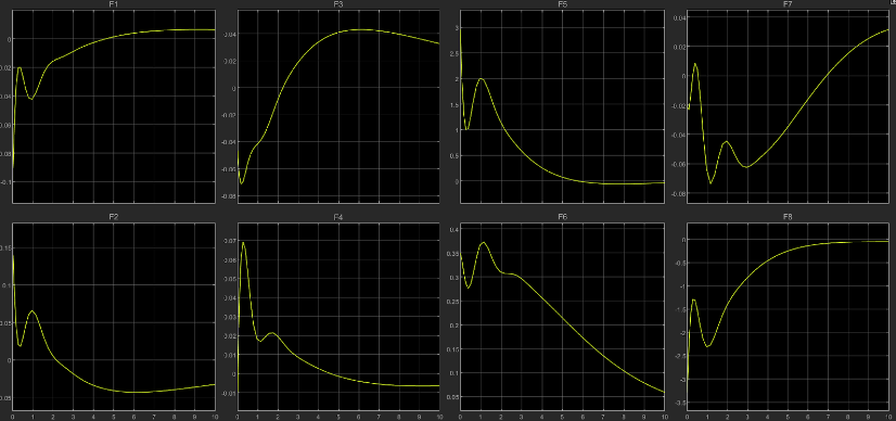
The controller input plots (controller input for each thruster will be as follows):

So, we can see that the thrust control input for thrusters 5,6,7 and 8 will be: \(-1.375*10^{-2}, 1.375*10^{-2}, 1.375*10^{-2}, -1.375*10^{-2}\) respectively.

Now, since propeller pair of 5 and 8 will be opposite to that of the pair 6 and 7, we get the total thrust on the ROV in Z-direction as: \(-1.375*10^{-2}*4*40 = 2N\) (approx.), where 40 is the gain.

So, the force in the vertical direction is balanced.

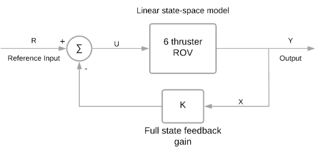
LQR Controller

Literature Review

The PID controller has been one of the most commonly used controllers for a really long time. There have been numerous PID tuning techniques, such as the Ziegler-Nichols method but are insufficient for high-performance control applications. The Linear Quadratic Regulator (LQR) is an optimal control method based on full state feedback. It aims to minimise the quadratic cost function and is then applied to linear systems, hence the name Linear Quadratic Regulator.

Why LQR controller?

The use of LQR  over PID control comes from the higher robustness of the former in terms of tuning the parameters with varying conditions. PID control uses the error in the input parameter of the closed loop system and tunes the parameters to reduce the error to zero. LQR, on the other hand, uses the state space model of the system and takes complete state feedback: -Kx, to calculate the error. LQR uses the method of cost function to calculate the control input cost vs the importance of achieving desired states.

State-Space Model with Full State Feedback Gain

\[\dot{X}=AX+BU\] \[y=CX+DU\]

Cost Function

The cost function defined by the system equations is minimised by the LQR controller using an optimal control algorithm. The cost function involves the system’s state parameters and input (control) parameters, along with the Q and R matrices. For the optimal LQR solution, the overall cost function must be as low as possible. The weights given to the state and control parameters are represented by the Q and R matrices, which act as knobs whose values can be varied to adjust the total value of the cost function.

The system must have a linearized state-space model to solve the LQR optimization problem. The cost function to be optimised is given by

\[J=\int{(X^TQX+U^TRU) dt}\]

Algebraic Riccati Equation and Its Solution ($S$ matrix)

The Q and R matrices are used to solve the Algebraic Riccati Equation (ARE) to compute the full state feedback matrix.

\[A^TS+SA-SBR^{-1}B^TS+Q=0\]

On solving the above equation, we obtain the matrix $S$.

Feedback Gain (K) and Eigen Values from $S$ matrix

The matrix 𝑆 obtained from the above ARE is used to find the full state feedback gain matrix K using the relation,

\[K=R^{-1}B^TS\]

The control matrix U is then given by

\[U=-KX\]

Linearisation of a state-space model

The linearization of a state-space model is needed while using the LQR technique since it works on linear systems. In our case, the state space model is in the form: ẋ = f(x); where f(x) is a nonlinear function of x. In such cases, to linearise the equation, we use the concept of linearising about a fixed point. The steps for the same are as follows:

1. Find the fixed points $\bar{x}$; where $f(\bar{x})=0.$
2. Linearise about an x̄, by calculating the Jacobian of dynamics at the fixed point x̄; where the latter can be represented as:

\[\mathbf{J}=\left[\begin{array}{ccc}\frac{\partial \mathbf{f}}{\partial x_1} & \cdots & \frac{\partial \mathbf{f}}{\partial x_n}\end{array}\right]=\left[\begin{array}{c}\nabla^{\mathrm{T}} f_1 \\\vdots \\\nabla^{\mathrm{T}} f_m\end{array}\right]=\left[\begin{array}{ccc}\frac{\partial f_1}{\partial x_1} & \cdots & \frac{\partial f_1}{\partial x_n} \\\vdots & \ddots & \vdots \\\frac{\partial f_m}{\partial x_1} & \cdots & \frac{\partial f_m}{\partial x_n}\end{array}\right]\]

where each term is a partial derivative of the dynamics with respect to a variable.

This step is executed since the dynamics of a nonlinear system behave linearly at the fixed point, or, in a small neighbourhood around the fixed point.

Changing the frame of reference to one with x̄ as the origin:

\[\dot{x} - \bar{\dot{x}} = f(x) \newline = f(\bar{x}) + J.(x-\bar{x})+J^2.{(x-\bar{x})}^2 + ....\]

where $J$ is calculated at $\bar{x}$.

The higher order terms from the third term $J^2.{(x-\bar{x})}^2$ are neglected since they are really small, hence the equation reduces to:

∆ẋ = 0 +J.∆x + 0

⇒ ∆ẋ = J.∆x

\[\Delta\dot{x} = 0+ J.\Delta x + 0 \newline = J.\Delta x\]

This is in the form $\dot{x} = Ax$.

Note: The above method for linearization works only when the fixed point satisfies the condition for linearising a system given by the Hartman Grobman Theorem, which states that:

“the behaviour of a dynamical system in a domain near a hyperbolic equilibrium point is qualitatively the same as the behaviour of its linearisation near this equilibrium point, where hyperbolicity means that no eigenvalue of the linearisation has real part equal to zero. Therefore, when dealing with such dynamical systems one can use the simpler linearisation of the system to analyse its behaviour around equilibria.[1]”

Hence, linearization works only when the fixed point is hyperbolic or put simply, has a non-zero real part.

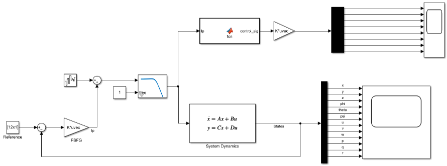
LQR Implementation

The following is the Simulink model that we built:

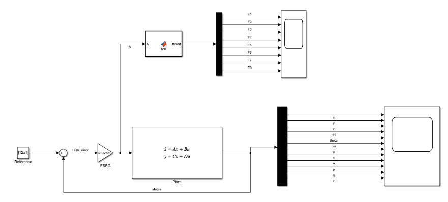
To implement this, we need the following:

1. State-space model:
   1. A and B matrices: These relate the derivative of the states with the current states and the control input. But, since our model is non-linear in nature, we cannot get a direct relation consisting of A and B matrices. Also, the LQR controller works only for Linear Systems. So, we have to linearise our system around an operating point. For our system, we took the origin in the world frame (initial point of the bot) as the operating point. Also, we used the position of the bot in the world frame and velocity of the bot in its own frame as the two states. Meaning:
   \[x = \begin{bmatrix} \eta \newline v \end{bmatrix}\]

(Here $x$ is the state but not the distance in x direction)

\[\begin{aligned}\dot{\boldsymbol{x}} & =\left[\begin{array}{c}\dot{\boldsymbol{\eta}} \\\dot{\boldsymbol{v}}\end{array}\right]=f\left(\boldsymbol{x}, \boldsymbol{u}, \boldsymbol{\tau}_d, t\right) \\& =\left[\begin{array}{c}J(\eta) \boldsymbol{v} \\M^{-1}\left[K p(A \boldsymbol{u})+\tau_d-C(\boldsymbol{v}) \boldsymbol{v}-D(\boldsymbol{v}) \boldsymbol{v}-g(\boldsymbol{\eta})\right]\end{array}\right]\end{aligned}\]

Since,

\[\dot{\eta} = J(\eta)v\]

The above state space model is clearly non-linear. So, we have to linearise to find A and B as follows:

\[A(t) \equiv\left[\begin{array}{cccc}\frac{\partial f_1}{\partial x_1} & \frac{\partial f_1}{\partial x_2} & \cdots & \frac{\partial f_1}{\partial x_n} \\\frac{\partial f_2}{\partial x_1} & \frac{\partial f_2}{\partial x_2} & \cdots & \frac{\partial f_2}{\partial x_n} \\& \vdots & \\\frac{\partial f_n}{\partial x_1} & \frac{\partial f_n}{\partial x_2} & \cdots & \frac{\partial f_n}{\partial x_n}\end{array}\right]_0 \newline \newline B(t) \equiv\left[\begin{array}{cccc}\frac{\partial f_1}{\partial u_1} & \frac{\partial f_1}{\partial u_2} & \cdots & \frac{\partial f_1}{\partial u_m} \\ \frac{\partial f_2}{\partial u_1} & \frac{\partial f_2}{\partial u_2} & \cdots & \frac{\partial f_2}{\partial u_m} \\ & \vdots & \\ \frac{\partial f_n}{\partial u_1} & \frac{\partial f_n}{\partial u_2} & \cdots & \frac{\partial f_n}{\partial u_m}\end{array}\right]_0\]

So, we obtain the A and B as follows:

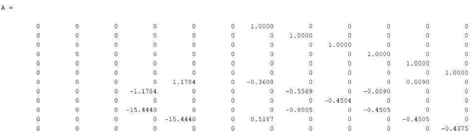
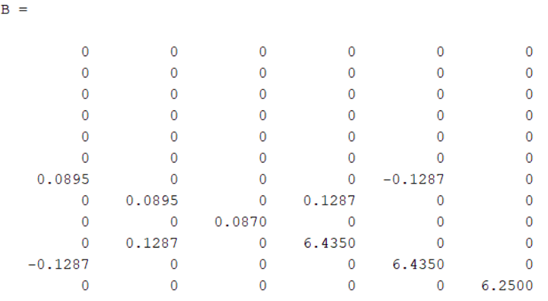
But we obtained the above results by taking weight W and buoyancy B as 110 N and 120 N respectively.

1. We take the C matrix in state-space $y = CX+DU$ as $eye(12)$ so as to send back all the states as feedback to the summing point.
2. Q and R matrices:
   1. Q stands for the importance of the states to reach their desired values.
   2. R stands for the cost of the control input.
   3. So, if we have an expensive control input compared to that of our needs to reach the states, we take the Q matrix to be dominating compared to R and vice versa.
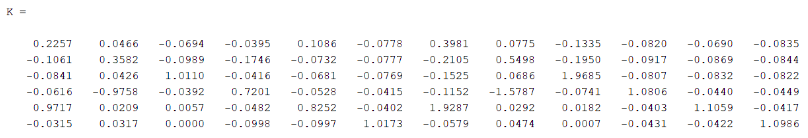
3. Then, we calculate the full-state feedback matrix, the Algebraic Riccati Equation and the eigenvalues by using the following command:

\[[K,S,P] = lqr(A,B,Q,R)\]

1. Then, we put the obtained value of the Gain matrix in the state-space model in Simulink. The following results are obtained for different R matrices (Q matrix being a 12x12 identity matrix) and desired states being $[1;2;1;[0;0;0;0;0;0;0;0;0]]$:

\[R = \begin{bmatrix}1 & 0.1 & 0.1 & 0.1 &0.1 &0.1 \\ 0.1 & 1 & 0.1 & 0.1 &0.1 &0.1\\ 0.1 & 0.1 & 1 & 0.1 &0.1 &0.1\\ 0.1 & 0.1 & 0.1 & 1 &0.1 &0.1\\ 0.1 & 0.1 & 0.1 & 0.1 &1 &0.1\\ 0.1 & 0.1 & 0.1 & 0.1 &0.1 &1 \end{bmatrix}\]

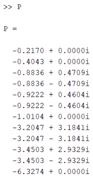
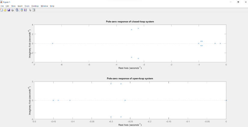
For the above, the Poles of the closed loop and open loop transfer function are as follows:

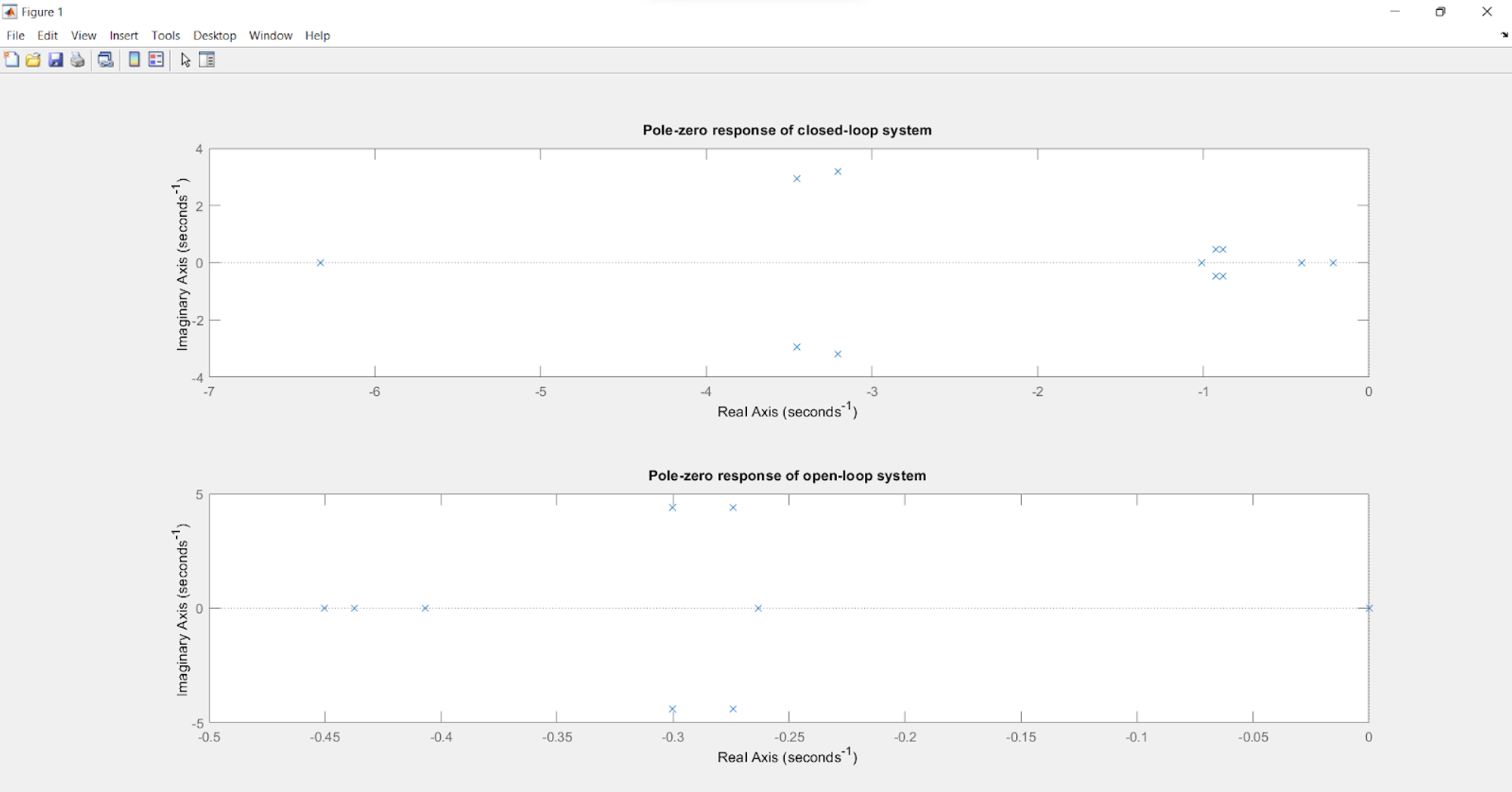
Poles:

Closed loop (With the feedback):

Open loop (Without the feedback):

Making ‘R’ more dominant

\[R = \begin{bmatrix}3 & 1.1 & 1.1 & 1.1 &1.1 &1.1 \\ 1.1 & 3 & 1.1 & 1.1 &1.1 &1.1\\ 1.1 & 1.1 & 3 & 1.1 &1.1 &1.1\\ 1.1 & 1.1 & 1.1 & 3 &1.1 &1.1\\ 1.1 & 1.1 & 1.1 & 1.1 &3 &1.1\\ 1.1 & 1.1 & 1.1 & 1.1 &1.1 &3 \end{bmatrix}\]

Making ‘R’ less dominant

\[R = \begin{bmatrix}0.11 & 0.01 & 0.01 & 0.01 &0.01 &0.01 \\ 0.01 & 0.11 & 0.01 & 0.01 &0.01 &0.01\\ 0.01 & 0.01 & 0.11 & 0.01 &0.01 &0.01\\ 0.01 & 0.01 & 0.01 & 0.11 &0.01 &0.01\\ 0.01 & 0.01 & 0.01 & 0.01 &0.11 &0.01\\ 0.01 & 0.01 & 0.01 & 0.01 &0.01 &0.11 \end{bmatrix}\]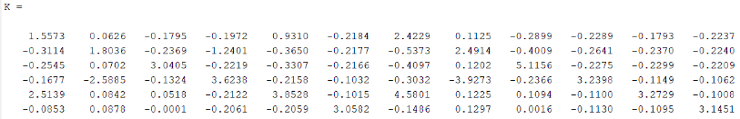

Results

1. Observed states:

More dominant ‘R’

Less dominant ‘R’

Thrust i/p to the thrusters:

More dominant ‘R’

Less dominant ‘R’

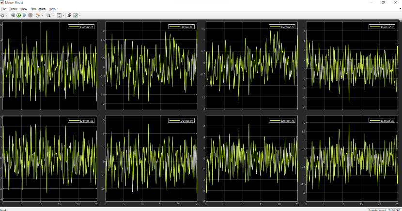
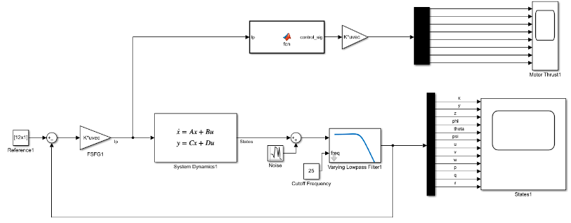
Band Limited White Noise

We planned on modelling a system with White Noise. So, we used the following control system:

Where:

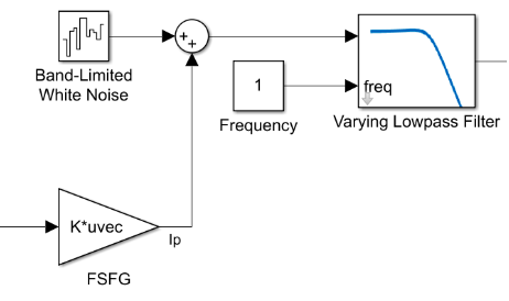
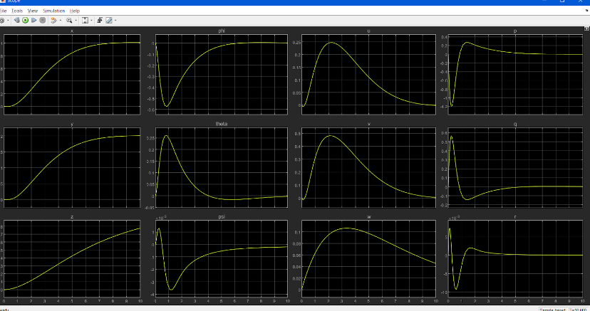
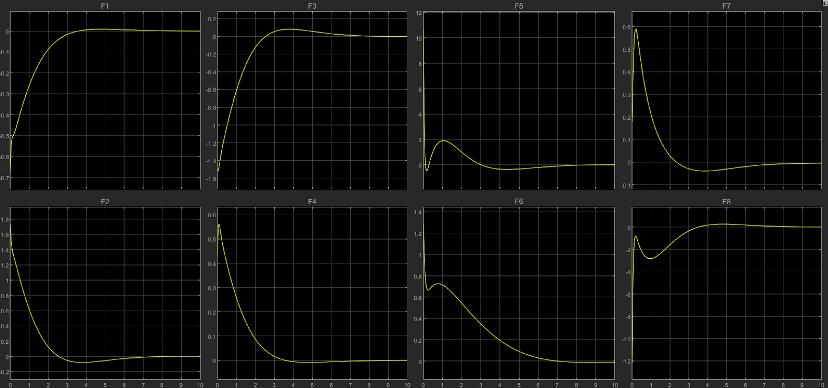
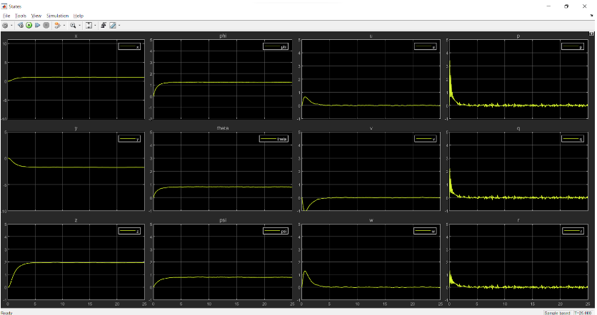
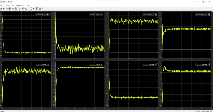
We included a low pass filter for removing noise with frequency greater than 1Hz. With low values of ‘Q’ we are getting really unstable results as the importance to the states is reduced. Later, we increased the value of Q to allow the states to reach quickly. This made the response of our system better. Taking the reference input as: [0;0;2;1.57;1;0.8;0;0;0;0;0;0];

1. $Q = eye(12):$

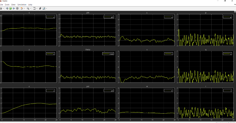
States:

Thrust provided by each thruster:

Poles of this system:

$Q = 1000*eye(12)$:

States:

Thrust provided by each thruster:

Poles of this system:

Clearly, the response of the system is faster in the second case.

Note: In the above two cases, the open loop and closed loop pole plots are drawn without taking the noise into account. The effect of noise is shown only in the ‘Thrust’ and ‘States’ plots.

Also, in the paper that we referred to, they considered noise caused due to the ‘current velocity’ which has a direct effect on the velocity of the rover instead of the torques. So, for that, a Random Number generator block was included in  the model as follows:

The parameters of the noise block are as follows:

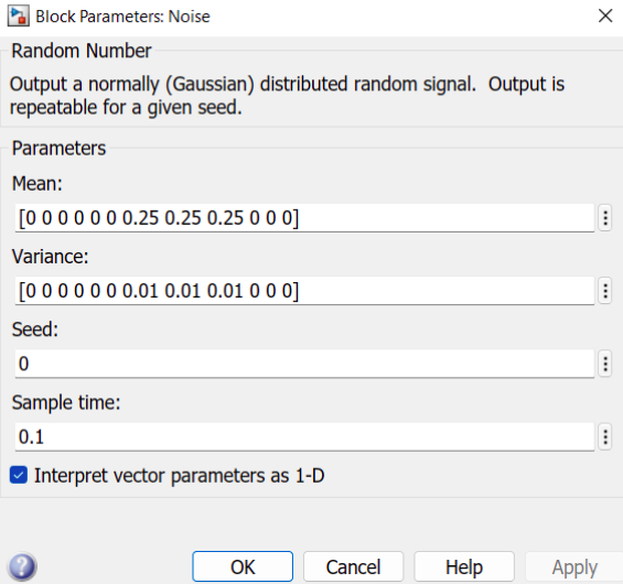
Here, noise is added considering the velocity of current as: $[0.25,0.25,0.25]$ and taking the variance as 0.01 in all the three directions.

Taking R matrix as: \(R = 1.2*eye(6)+0.8*ones(6)\)

And Q matrix as: $Q = 1000*eye(12)$

The results that we obtained for 1 min stop time are:

States:

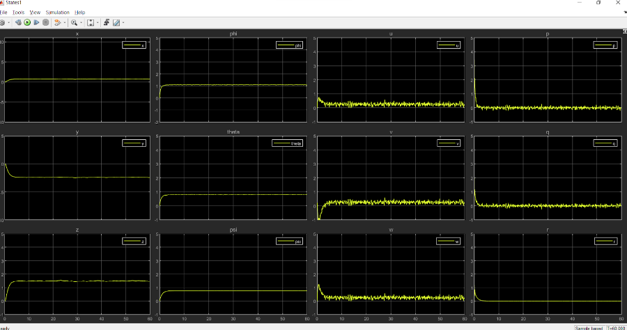
Thrust provided by each thruster:

Clearly, the thrust output involves too much vibrations.

Analysis of Eigenvalues

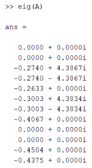
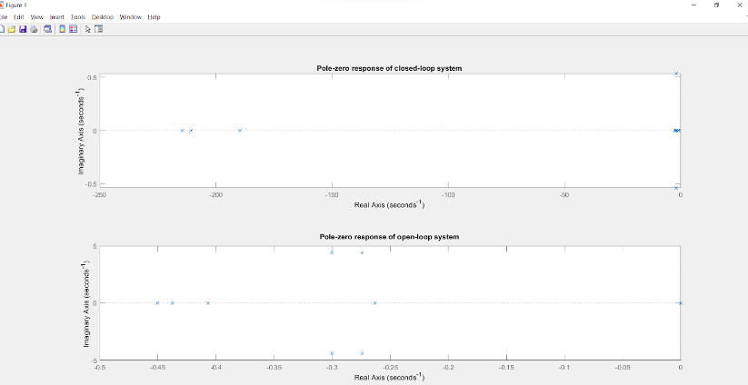
When we analyse the change in eigen values while considering the open loop and LQR controlled closed loop systems, for the same values of Q,R we see a clear change in their position in the pole zero plot.

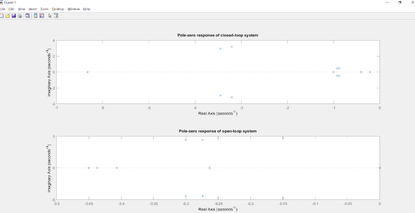
Considering the above plot, we can see a clear shift in the eigen values in the direction of the negative real axis, ensuring more stability of the system. As we write down the eigen values or the poles of the two systems, the difference becomes evident.

For $Q=eye(12)$ & \(R = 0.1*ones(12)+0.9*eye(12)\)

Open loop poles	Closed loop poles
0.0000 + 0.0000i	-6.3274 + 0.0000i
0.0000 + 0.0000i	-3.2047 + 3.1841i
-0.2740 + 4.3867i	-3.2047 - 3.1841i
-0.2740 - 4.3867i	-3.4503 + 2.9329i
-0.2633 + 0.0000i	-3.4503 - 2.9329i
-0.3003 + 4.3834i	-0.9222 + 0.4604i
-0.3003 - 4.3834i	-0.9222 - 0.4604i
-0.4067 + 0.0000i	-0.8836 + 0.4709i
0.0000 + 0.0000i	-0.8836 - 0.4709i
0.0000 + 0.0000i	-1.0104 + 0.0000i
-0.4504 + 0.0000i	-0.2170 + 0.0000i
-0.4375 + 0.0000i	-0.4043 + 0.0000i

As it can be observed, in the case of the open loop system, we have four eigen values or poles located at the origin which leads to the fact that the system is marginally stable. Whereas, for the closed loop system, most of  the poles have shifted towards the left side of the imaginary axis with all the poles lying on the left half of the s-plane. This gives enough proof to say that after implementing LQR control, the system has become more stable as compared to the open loop system and hence has helped in increasing performance in terms of reaching the end states.

Conclusion

Given the results of implementing both PID and LQR control on the ROV system, we can see a better response for an LQR control over the PID when we include disturbances in the environment. Also, the LQR control is far more robust in adapting to the change in buoyancy as compared to the PID control, which broadens the spectrum of usage in the former as compared to the latter. When we have changes in the system, using a PID requires tuning all the three gain values for all the control inputs. Tuning the gain values for multiple parameters is not an easy task and there is a very narrow range of values which give the desired results for a specific situation. On the other hand, when we want to adapt to changes while working on LQR control, our tuning is dependent only on the Q,R cost matrices which can help in changing the  relative importance of the states and control inputs for a given circumstance. Here, our goal is achieved by changing the values of the matrices, so as to select the more important factor among the states and inputs,  where we achieve the desired results for a wide range of values which only differ in terms of speed of transient response and steady state error. Another advantage of LQR over PID control that we have come across was the ability to easily control velocity components along with the position coordinates, which would lead to much more complexity in the case of a PID based controller. For simulating in a noisy environment, we used nonlinear PID control where a water current velocity was added as a disturbance; its value being constant with time and we attained appreciable results. Whereas for the LQR setup, we have used a gaussian white noise as a source of disturbance, which gives a better look at the real world scenario. Upon increasing the Q matrix or simply, the cost of attaining the states, we have observed better performance in attaining the states and less erratic, more uniform thrust outputs produced by the thrusters; which is a more reliable result since it is realisable in a real world environment.

However, one drawback of using the LQR control is its applicability to only linear systems, whereas most of the real world scenarios tend to have non linearity in them. However, this problem can be overcome by linearising the system near the fixed points and applying the control.

Hence, we have come to the conclusion that using an LQR control is far more reliable than a PID control for the positional and velocity control of a 6-DOF Autonomous Underwater Vehicle.

Future Work

• The model can be implemented with an Adaptive Controller based system which is expected to give better performance.
• We wish to implement our work on the actual physical system to know how it works in the real world. And by doing that, we will be able to understand how the sensor noise affects the system and how the controller will compensate for it.