Path Planning

Resources

Programming

Path Planning

Path planning, also known as motion planning, is the process of finding a feasible path from a starting point to a desired goal point while avoiding obstacles in between. This is a fundamental problem in robotics, automation, and computer graphics.

There are several types of algorithms used for path planning:

1. Visibility graph algorithm: This algorithm constructs a graph of visibility between the starting point, the goal point, and all obstacles. The nodes of the graph are the starting point, goal point, and the vertices of the obstacles. The edges of the graph connect nodes that have a clear line of sight. This graph is then used to find the shortest path between the starting point and the goal point.
2. Random-exploring algorithms: These algorithms randomly sample the configuration space (the space in which the robot can move) to find a path from the starting point to the goal point. Examples of random-exploring algorithms include Rapidly-exploring Random Trees (RRT) and Probabilistic Roadmaps (PRM).
3. Optimal search algorithms: These algorithms use a search strategy to find the optimal path from the starting point to the goal point. Examples of optimal search algorithms include A* (A-star), Dijkstra’s algorithm, and Breadth-First Search (BFS). These algorithms use heuristics or cost functions to guide the search towards the goal point while minimizing the path length.

Autonomy requires that the robot is able to plan a collision-free motion from an initial to a final posture on the basis of geometric information.

Information about the workspace geometry can be

• entirely known in advance, called off-line planning
• gradually discovered by the robot, called on-line planning

Discrete Planning

They are the simplest to describe because the state space will be finite (or countably infinite) in most cases. No forms of uncertainty will be considered.

Formulation:

1. A nonempty state space X, with finite or countably infinite set of states.
2. For each state $x \in X$, a finite action space $U(x).$
3. A state transition function $f$ that produces a state $f(x,u) \in X$ for every $x \in X$ and $u \in U(x)$. The state transition equation is given by $x’=f(x,u)$.
4. An initial state $x_I \in X.$
5. A goal set $X_G \subset X.$

General Forward Search

Pseudo code:

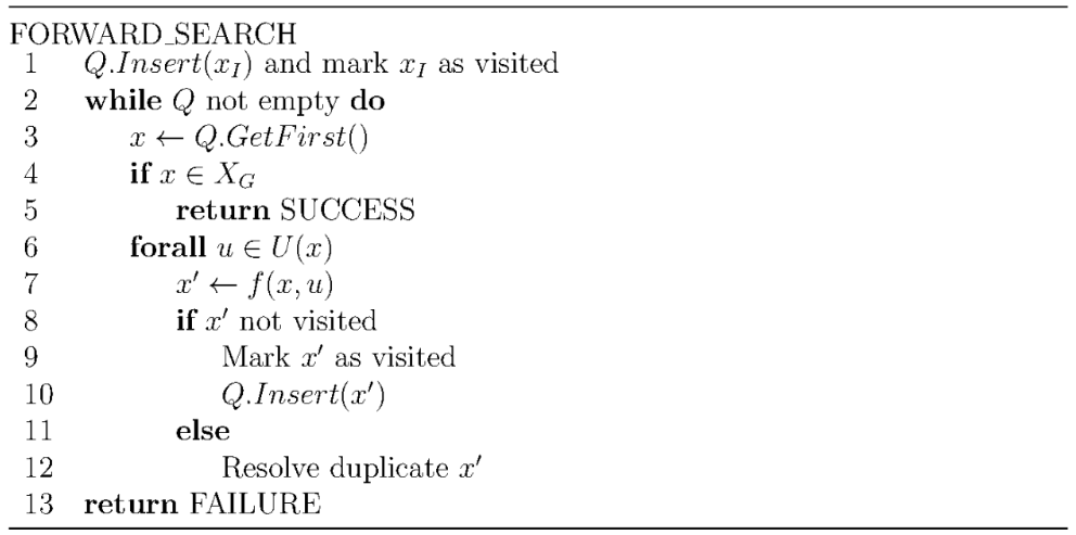
The set of alive states is stored in a priority queue, Q, for which a priority function must be specified. The only significant difference between various search algorithms is the particular function used to sort Q. Therefore, assume for now that Q is a common FIFO (First-In First-Out) queue; whichever state has been waiting the longest will be chosen when $Q.GetFirst()$ is called. Initially, Q contains the initial state $x_I$. A while loop is then executed, which terminates only when Q is empty. This will only occur when the entire graph has been explored without finding any goal states, which results in a FAILURE (unless the reachable portion of X is infinite, in which case the algorithm should never terminate). In each while iteration, the highest ranked element, x, of Q is removed. If $x$ lies in $X_G$, then it reports SUCCESS and terminates; otherwise, the algorithm tries applying every possible action, $u \in U(x)$. For each next state, x’ = f(x,u), it must determine whether x’ is being encountered for the first time. If it is unvisited, then it is inserted into Q; otherwise, there is no need to consider it because it must be either dead or already in Q.

Breadth First

Breadth-First Forward Search (BFS) is a graph traversal algorithm that systematically explores all the vertices (or nodes) of a graph in a breadth-first order, i.e., visiting all nodes at the same level before moving on to the next level.

The algorithm starts by visiting the root node (or starting node) and then visits all the nodes at the next level before moving on to the nodes at the next level, and so on until all nodes have been visited. It uses a FIFO queue data structure to keep track of the nodes that have been visited but whose neighbors have not yet been visited. The queue is initialized with the root node, and the algorithm iteratively dequeues a node, visits all its neighbors, and enqueues them if they have not been visited before.

The time complexity of BFS is $O(V+E)$, where V is the number of vertices (nodes) in the graph, and E is the number of edges. This is because the algorithm visits each node and each edge at most once. Also, $V=X, E=UX$ if the same actions U are available from every state. It is systematic. The worst-case performance of BFS is worse than that of A* and dynamic programming.

Pseudo code:

1. Initialise a queue data structure with the root node.
2. Mark the root node as visited.
3. Dequeue a node from the queue and visit it.
4. Enqueue all the unvisited neighbors of the node.
5. Mark all the enqueued neighbours as visited.
6. Repeat steps 3-5 until the queue is empty.

function BFS(start_node):
    Q = Queue()  // Initialize a queue
    Q.enqueue(start_node)  // Enqueue the start node
    visited = set()  // Initialize a set of visited nodes
    while not Q.empty():  // While the queue is not empty
        node = Q.dequeue()  // Dequeue the next node
        if node not in visited:  // If the node has not been visited
            visited.add(node)  // Mark the node as visited
            // Process the node (e.g., print its value)
            print(node)
            // Enqueue all unvisited neighbors of the node
            for neighbor in get_neighbors(node):
                if neighbor not in visited:
                    Q.enqueue(neighbor)

Depth First

Depth First Forward Search (DFS) is a graph traversal algorithm that explores the vertices of a graph in a depth-first manner, starting from a given source vertex, and visiting all the vertices reachable from it.

The DFS algorithm can be implemented using a LIFO stack data structure to keep track of the vertices being explored. When a vertex is visited, it is pushed onto the stack, and its unvisited neighbours are added to the stack in the order in which they are encountered. When there are no more unvisited neighbours, the vertex at the top of the stack is popped off and the algorithm backtracks to the previous vertex.

The time complexity of DFS algorithm is $O(V+E)$, where V is the number of vertices in the graph and E is the number of edges. The space complexity of the algorithm is O(V) due to the stack used to keep track of the visited vertices. It is systematic. The search could easily focus on one direction and completely miss large portions of the search space as the number of iterations tends to infinity.

Pseudo code:

1. Start at the source vertex.
2. Mark the source vertex as visited.
3. Explore each unvisited neighbor of the source vertex in depth-first order.
4. When there are no more unvisited neighbors, backtrack to the previous vertex and repeat step 3 for its unvisited neighbors.
5. Continue this process until all reachable vertices have been visited.

function depthFirstForwardSearch(graph, source):
    // Initialize a stack for DFS traversal and a set to keep track of visited vertices
    stack = new Stack()
    visited = new Set()

    // Push the source vertex onto the stack and mark it as visited
    stack.push(source)
    visited.add(source)

    while not stack.isEmpty():
        // Pop the top vertex from the stack and print it
        currentVertex = stack.pop()
        print currentVertex

        // Explore the neighbors of the current vertex
        for neighbor in graph.getNeighbors(currentVertex):
            if neighbor not in visited:
                // Push the neighbor onto the stack and mark it as visited
                stack.push(neighbor)
                visited.add(neighbor)

Best First

Best First search is a heuristic search algorithm that is used to find the optimal path between two points in a graph. The algorithm expands the node with the lowest heuristic value first, i.e., the node that appears to be the closest to the goal. The search starts from the initial state and moves towards the goal state. It uses a heuristic function h(n) to evaluate the distance between a node n and the goal state. The algorithm maintains a priority queue (or a heap) of the nodes to be expanded, with the node with the lowest heuristic value at the front of the queue. It is not systematic.

Pseudo code:

1. Initialise the open list with the start node as the only element.
2. Initialise the closed list as an empty set.
3. While the open list is not empty, do the following:
   • Remove the node with the lowest heuristic value from the open list.
   • If the removed node is the goal node, return the path.
   • Otherwise, expand the node by generating all its neighbouring nodes.
   • For each neighbouring node, calculate its heuristic value h(n) and add it to the open list if it is not already in the closed list or the open list.
   • Add the expanded node to the closed list.
4. If the open list becomes empty and the goal node is not found, return failure.

Iterative Deepening

Iterative Deepening Algorithm (IDA) is a general search algorithm based on depth-first search (DFS), but unlike DFS, IDA performs multiple iterations, each with increasing depth limits. The algorithm starts with a depth limit of one and iteratively increases it until the goal is found.

The iterative deepening algorithm uses a breadth-first search-like strategy to incrementally search the space by exploring each level of the search tree. The algorithm starts by searching the tree at a depth limit of one. If the goal is not found, the algorithm increases the depth limit to two and searches the tree again. This process is repeated until the goal is found.

The iterative deepening algorithm is often used in cases where the search space is too large for a complete search. By limiting the search depth, the algorithm can focus on the most promising parts of the search space, while still being able to find the optimal solution. The time complexity of IDA is O(b^d), where b is the branching factor and d is the depth of the goal node. The space complexity of the algorithm is O(d). It has better worst-case performance than BFS. Furthermore, the space requirements are reduced because the queue in BFS is usually much larger than for DFS.

Combinatorial Motion Planning

Roadmap Based Path Planning: Visibility Graph and Generalised Voronoi Diagrams as roadmaps

Covers visibility graphs and voronoi diagrams.

Combinatorial motion planning is a subfield of robotics and artificial intelligence that focuses on developing algorithms and techniques for planning the motion of robots in complex environments. The goal is to find feasible paths that enable robots to reach their desired goals while avoiding obstacles and adhering to various constraints.

Unlike continuous motion planning, which deals with continuous trajectories, combinatorial motion planning involves searching through a discrete set of possible motions and selecting the optimal one. This involves exploring the space of all possible robot configurations and determining which configurations can be reached without colliding with obstacles or violating constraints.

Some common techniques used in combinatorial motion planning include graph-based search algorithms, sampling-based planners, and cell decomposition methods. These techniques leverage computational tools and mathematical models to efficiently plan the motion of robots and ensure they operate safely and effectively.

Continuous Motion Planning Methods

Continuous motion planning methods are algorithms and techniques used to plan the continuous motion of robots in complex environments. Unlike combinatorial motion planning, which deals with a discrete set of possible motions, continuous motion planning deals with continuous trajectories.

Continuous motion planning methods use mathematical models and algorithms to determine optimal trajectories that enable robots to reach their desired goals while avoiding obstacles and adhering to various constraints. These methods often involve the use of calculus and optimization techniques to find the optimal path.

They are often more computationally intensive than combinatorial motion planning methods. This is because they involve solving complex mathematical equations and optimizing continuous functions. However, they offer greater flexibility and precision in planning robot motion, enabling robots to operate more efficiently and effectively in complex environments.

Examples of continuous motion planning techniques include:

1. Trajectory optimization: This method involves finding the optimal trajectory for a robot by solving an optimization problem that minimizes a cost function. The cost function can be customized to include constraints on the robot’s motion, such as collision avoidance or energy consumption. Trajectory optimization can be solved using numerical optimization techniques, such as gradient descent or nonlinear programming.
2. Control-based planning: This method involves using a control law to steer the robot along a desired trajectory. The control law can be designed using various techniques, such as feedback linearization or model predictive control. Control-based planning can be used to plan the motion of robots in dynamic environments, where the robot’s motion must be continuously updated in response to changing conditions.
3. Model predictive control (MPC): MPC is a control-based planning method that involves predicting the future behavior of the robot and optimizing its motion accordingly. MPC uses a dynamic model of the robot and the environment to predict how the robot’s motion will affect its surroundings, and it optimizes the robot’s motion to achieve a desired goal while satisfying various constraints.
4. Sampling-based planning: This method involves randomly sampling the robot’s configuration space to generate a set of feasible trajectories. The set of trajectories is then pruned to remove those that collide with obstacles or violate constraints. Sampling-based planning is computationally efficient and can be used to plan the motion of robots in high-dimensional spaces, but it may not always find the optimal trajectory.

Roadmaps

Roadmaps in combinatorial motion planning refer to a set of interconnected nodes and edges that are constructed in the configuration space of a robot or a group of robots. The configuration space represents all possible configurations of the robot(s) in the environment, including their position, orientation, and other relevant parameters.

The roadmap construction process involves sampling the configuration space and identifying collision-free configurations that can be used as nodes in the roadmap. These nodes are then connected by edges that represent feasible paths between them. The resulting roadmap provides a discrete representation of the configuration space and enables efficient path planning for the robot(s).

There are several types of roadmaps that can be used in combinatorial motion planning, including probabilistic roadmaps (PRMs), visibility graphs, and cell decomposition-based roadmaps. Each type has its strengths and weaknesses, and the choice of roadmap depends on the specific application and requirements.

There are many roadmap-based approaches, and they primarily fall into 3 categories:

1. Topological Model - Every location is represented by a node, which are connected by edges.
2. Geometrical Model - The geometry of the environment, containing obstacles, is considered and a free space, which is a collection of all free configurations that do not collide with the obstacles, is created.
3. Grid-based Model - The entire environment is divided in cells or grids and based on the connectivity between these grids, roadmaps are created.

Formal definition: A union of one dimensional curves R is a roadmap if for all starting positions q and goal positions g, that can be connected by a path, the following properties hold -

• Accessibility - There exists a path from q to some point q’ on R
• Departability - There exists a path from a point g’ on R to g
• Connectivity - There exists a path in R from q’ to g’

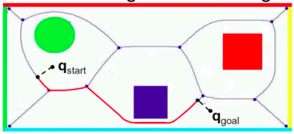
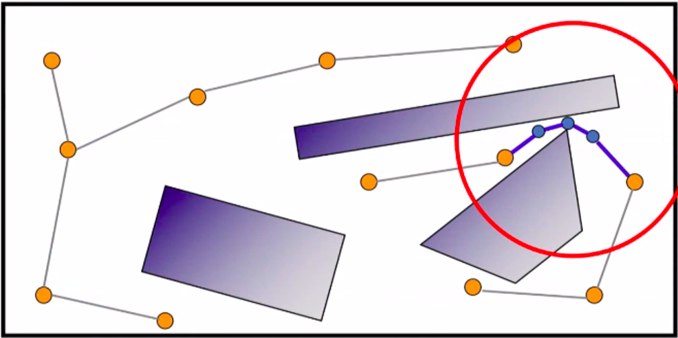
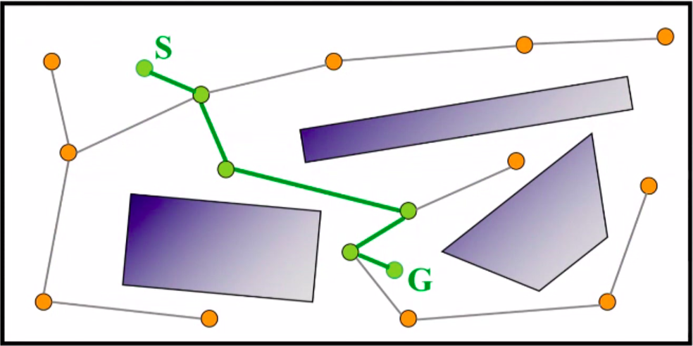
Visibility Graph

The visibility graph is a method used to represent the connectivity of a configuration space. A configuration space is the space that represents all possible positions and orientations of a robot or object.

The basic idea is that if we stretched a rubber band from start to target, weaving in and out of the obstacles, the band would form a straight line between the obstacles, and would wrap around the obstacles themselves.

The visibility graph is constructed by first placing a node at each obstacle boundary and at the starting and ending configurations of the robot. Then, an edge is added between two nodes if the line segment connecting them does not intersect any obstacle boundaries. This process creates a graph that represents all possible paths that the robot can take without colliding with any obstacles. Its edges are the edges of the obstacles and edges joining all pairs of vertices that can see each other.

It is based on the principle that given a start point and a goal point, we look for all vertices of obstacles present in the environment which are visible from the given start location. We then traverse through those vertices to reach the destination in the shortest path.

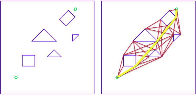
Start, goal, vertices of obstacles are graph nodes. Edges are “visible” connections between nodes, including obstacle edges.

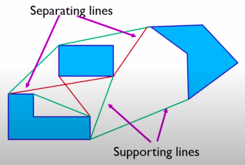
Reduced Visibility Graph

A reduced visibility graph consists of very few edges to reduce its complexity. It makes use of supporting and separating lines.

• Supporting lines are edges in the visibility graph that connect two vertices on the boundary of the same obstacle. The obstacles lie on the same side of the supporting lines. These edges are important because they represent the possibility of the robot following a path along the boundary of an obstacle without colliding with it. Supporting lines can be used to construct a continuous path for the robot along the boundary of an obstacle, which is useful in situations where the robot cannot pass through the obstacle.
• Separating lines, on the other hand, are edges in the visibility graph that connect two vertices on the boundaries of different obstacles. The obstacles lie on opposite sides of the separating lines. These edges represent the possibility of the robot moving between two obstacles without colliding with either one. Separating lines are important because they define the regions of the configuration space that are accessible to the robot, and can be used to divide the configuration space into different regions, each of which can be explored separately.

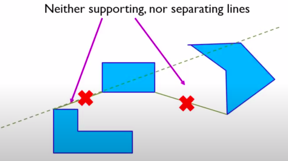
Neither supporting nor separating since they cut through the obstacles. They are avoided in constructing visibility graphs.

Rotational Plane Sweep Algorithm

It is used for constructing a visibility graph for a set of obstacles in a configuration space. The algorithm works by sweeping a ray around the configuration space and adding edges to the visibility graph whenever the ray intersects an obstacle boundary.

• Input: A set of vertices ${v_i}$(whose edges do not intersect) and a vertex v.
• Output: A subset of vertices from ${v_i}$ that are within the line of sight of v.

Pseudo code:

FOR each vertex v(i), calculate alpha(i)
NEW vertexSet = set of alpha(i) which are increasing order
NEW activeSet = set of edge which intersect the horizontal half line emanating from v
FOR all alpha(i)
	IF v(i) is visible v
		THEN visibleSet.PUSH(edge(v,v(i))
	ENDIF
	IF v(i) is the beginning of an edge, vertexSet, not in activeSet
		THEN activeSet.PUSH(vertexSet)
	ENDIF
	IF v(i) is the end of an edge in activeSet
		THEN activeSet.DELETE(edge(v(i), v))
	ENDIF
ENDFOR

Once the visibility graph is built, then robot starts to find the path among visibility graph. Since the visibility map posses the properties of accessibility and departability by definition, if it is connected, then several kinds of searching algrithm can be implemented such as potential function and various star algorithm. Cost between nodes can be set to distance of nodes and heuristic cost function can be set to estimated cost of shortest path from node to goal.

The shortest path being computed tries to stay as close as possible to the obstacles. Any execution error will lead to a collision. It also becomes more complex in higher dimensions.

Cell Decomposition

Cell decomposition is a technique used in combinatorial motion planning to divide the workspace into smaller regions, called cells, that can be easily navigated by a robot. Each cell is defined as a region that is either free of obstacles or contains a single obstacle.

The process of cell decomposition involves dividing the workspace into a grid of cells, where each cell is either classified as free or occupied by an obstacle. This grid can then be used to represent the workspace as a graph, where the cells are the nodes and the edges connect adjacent cells.

One advantage of cell decomposition is that it simplifies the motion planning problem by reducing it to a discrete search problem. It also allows for the use of graph-based algorithms, such as Dijkstra’s algorithm or A*, to find a path from the starting cell to the goal cell.

There are several types of cell decomposition techniques, including:

1. Voronoi Diagrams: These are diagrams that divide the workspace into regions based on the distance to the obstacles. The cells in a Voronoi diagram represent the regions of the workspace that are closest to a particular obstacle.
2. Binary Space Partitioning (BSP): This technique divides the workspace into two subspaces recursively, with each subspace divided by a line or plane. This creates a tree structure where each node represents a subspace and each leaf node represents a single cell.
3. Quadtree Decomposition: This technique recursively divides the workspace into four quadrants, with each quadrant further subdivided until each cell contains at most one obstacle.

Voronoi Diagram

Voronoi diagrams are a geometric structure that partition a space into a set of regions based on the distance to a given set of points or objects. In the context of motion planning, Voronoi diagrams can be used to represent the free space and obstacles in a configuration space, and to compute paths or trajectories for a robot navigating through that space.

The Voronoi diagram for a set of points in a space consists of a set of cells, where each cell represents the region of space that is closest to a particular point or object. The cells are defined by a set of lines or curves, called the Voronoi edges, which are equidistant from the neighboring points or objects. The Voronoi diagram is often visualized as a set of polygonal cells that cover the entire space, with the edges of the cells corresponding to the Voronoi edges.

Generalized Voronoi Diagrams

Robot Path Planning Using Generalized Voronoi Diagrams.

The obstacles in the real world are never points but they’re large objects. Generalized Voronoi Diagrams are just like regular VDs, but instead of the regions around points, we have the regions around objects.

Generalized Voronoi Graph

Create Voronoi regions with Python

Vertical Strip Cell Decomposition

• The cells joining the start and target are shaded.
• The resolution of the decomposition is chosen to get a collision-free path dependent on the sensitivity of controlling robot’s motion.

Planning

• Find the point \(q*_{start}\) of the Voronoi diagram closest to \(q_{start}\).
• Find the point \(q*_{goal}\) of the Voronoi diagram closest to \(q_{goal}\).
• Compute the shortest path from \(q*_{start}\) to \(q*_{goal}\) on the Voronoi diagram.

Sampling based Motion Planning

The state space for motion planning, C, is uncountably infinite. Yet a sampling based planning algorithm can consider at most a countable number of samples.

Single Query and Multi Query Planning

Multi-query path planning and single-query path planning are two different types of path planning algorithms used in robotics and computer science.

Single-query path planning refers to finding a path between two given points in a given environment, where the start and end points are fixed and do not change. In other words, it is the process of finding a path from a single source to a single destination in a given environment. This is a common problem in robotics, where robots need to navigate from one point to another without colliding with obstacles. It is only concerned about a portion of free C-space needed for a query.

On the other hand, multi-query path planning refers to finding paths between multiple pairs of points in a given environment. Unlike single-query path planning, in multi-query path planning, the start and end points can vary from one query to another. For example, a robot may need to navigate to different locations in a warehouse to pick up items, and the start and end points will change with each new task. Th goal is to efficiently model the entire C-space so as to answer any query in that space. Example - Probabilistic Roadmap (PRM)

Multi-query path planning is more complex than single-query path planning, as it requires the algorithm to efficiently handle multiple queries and avoid recalculating the entire path for each new query. However, it can be more efficient in situations where there are multiple tasks to be completed in the same environment.

Probabilistic Roadmap of Tree (PRT) combines both ideas.

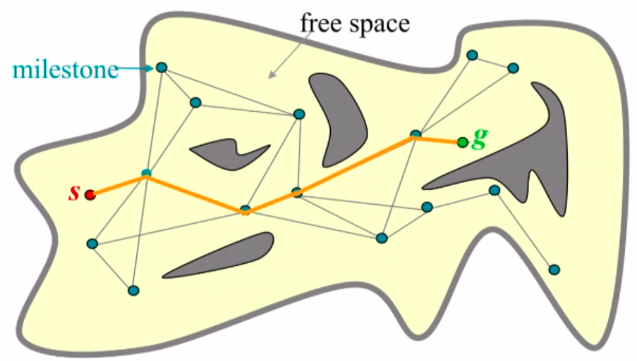
Probabilistic Roadmap (PRM)

It is a randomized algorithm that is designed to efficiently find collision-free paths for robots in complex environments. PRM algorithm involves the following components:

1. Roadmap construction: The first step of PRM is to construct a roadmap of the environment. This is done by randomly sampling configurations of the robot in the environment and checking whether they are collision-free. Collision-free configurations are added to the roadmap as nodes, and connections are made between nodes that are within a certain distance of each other.
   • Milestones: Milestones are the nodes in the roadmap that represent the important configurations of the robot in the environment. These configurations are sampled randomly from the configuration space of the robot, and they are checked for collision with the obstacles in the environment. If a configuration is collision-free, it is added as a milestone to the roadmap.
   • Local paths: Local paths are the edges that connect the milestones in the roadmap. They represent the feasible paths that the robot can take between the milestones. The local paths are computed by planning a short path between each pair of milestones, while avoiding the obstacles in the environment.
2. Roadmap search: The next step is to search the roadmap for a path between the start and goal configurations. The local paths are used to guide the robot along the roadmap, and the milestones serve as guideposts to ensure that the robot stays on a collision-free path. This is done using a standard graph search algorithm, such as A* search or Dijkstra’s algorithm. The algorithm tries to find the shortest path between the start and goal configurations while avoiding collisions with obstacles.
3. Path refinement: The final step is to refine the path found by the roadmap search. This is done by iteratively attempting to move along the path and checking for collisions. If a collision is detected, the path is locally modified to avoid the obstacle. This process continues until a collision-free path is found.

Features:

• PRMs don’t represent the entire free configuration space, but rather a roadmap through it.
• Roadmap is an undirected acyclic graph R = (N,E).
• Nodes N are robot configurations in free C-space, called milestones.
• Edges E represent local paths between configurations.
• Learning Phase
  • Construction: reasonably connected graph covering C-space
  • Expansion: improve connectivity
  • Local paths not memorized (cheap to re-compute)

Construction overview:

1. R = (N,E) begins empty
2. A random free configuration c is generated and added to N
3. Candidate neighbours to c are partitioned from N
4. Edges are created between these neighbours and c, such that acyclicity is preserved
5. Repeat 2-4 until done

General Local Planner:

1. Connect the two configurations is C-space with a straight line segment
2. Check the joint limits
3. Discretize the line segment into a sequence of configurations c1, c2, …, cm such that for every $(c_i, c_{i+1})$, no point on the robot at ci lies further than $\epsilon$ away from its position at ci+1
4. For each ci, grow robot by $\epsilon$, check for collisions

Edges are created between these neighbours and c, such that acyclicity is preserved.

Random Bounce Walk:

1. Pick a random direction of motion in C-space, move in this direction from c.
2. If collision occurs, pick a new direction and continue.
3. The final configuration n and the edge (c,n) are inserted into the graph.
4. Attempt to connect n to other nodes using the construction step technique.
5. Path between c and n must be stored, since process is non-deterministic.

Select c such that P(c is selected) = w(c)

Query Phase:

• Connect start and goal configurations to roadmap (say $\hat{s}$ and $\hat{g}$)
• Find path between $\hat{s}$ and $\hat{g}$ in roadmap

Pros:

• Once learning is done, queries can be executed quickly
• Complexity reduction over full C-space representation
• Adaptive - can incrementally build on roadmap
• Probabilisically complete, which is usually good enough

Cons:

• $\hat{s}$ and $\hat{g}$ should be in same connected component, else failure
• Paths are not optimal. They can be long and indirect, depending on how the graph was created. Smoothing can be applied.

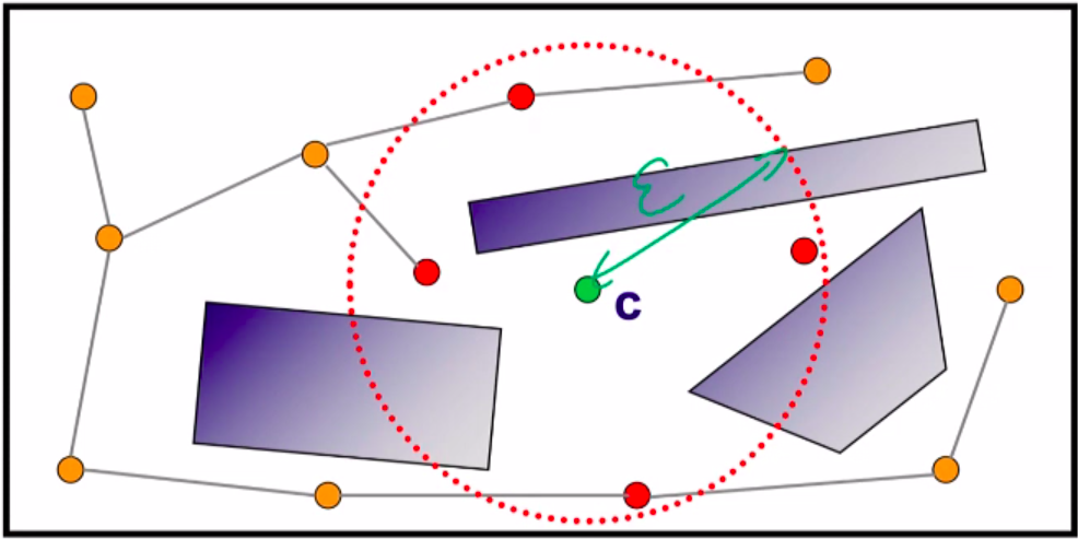
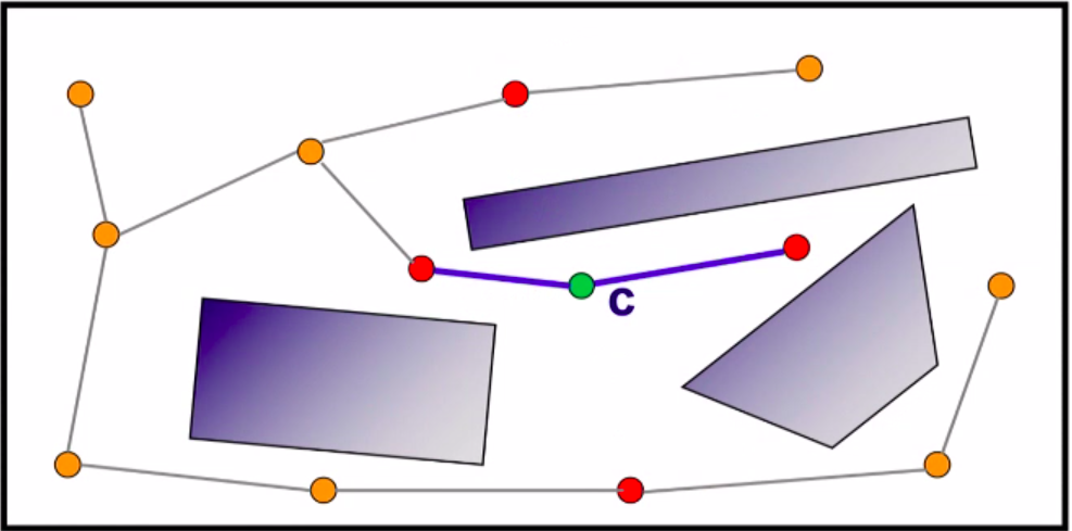
Rapidly-Exploring Random Tree (RRT)

[Path Planning with A* and RRT

Autonomous Navigation, Part 4](https://www.youtube.com/watch?v=QR3U1dgc5RE&t=45s)

RRT, RRT* & Random Trees

RRT is a probabilistic algorithm that builds a tree of feasible paths in the search space.

The RRT algorithm starts with an initial configuration of the robot or system being planned for, and then iteratively grows a tree by randomly selecting a new configuration, and connecting it to the closest node in the tree. The algorithm continues to grow the tree until a path is found from the initial configuration to the goal configuration, or until a certain maximum number of iterations is reached.

The random sampling and connection of nodes in RRT allows it to quickly explore large areas of the search space, making it well-suited for solving complex path planning problems in high-dimensional spaces. Additionally, RRT can handle non-holonomic constraints, as well as dynamic obstacles and changes in the environment.

RRT has several variants, including RRT* and RRT-Connect, which incorporate optimization and connectivity constraints to improve the quality of the resulting paths.

RRTs have the advantage that they expand very fast and bias towards unexplored regions of the configuration space and so covering a wide area in a reduced time.

When one of the leaves of the tree reaches a goal region, the algorithm stops and a path can directly be found by following the predecessors of the last added node.

Features:

• It is implemented using tree data structure
• Tree is special case of directed graph
• Edges are directed from child node to parent
• Every node has one parent, except root
• Nodes represent physical states or configurations
• Edges represent feasible paths between states
• Each edge has cost associated traversing feasible path

Pseudo code:

1. Initialize tree T with a single node at the start state S
2. while not goal_found and iterations < max_iterations do
3.     randomly sample a new configuration Q
4.     find the node N in T that is closest to Q
5.     extend the tree from N towards Q by a maximum distance delta_q
6.     if Q is within delta_q of the goal state G, add a node at Q and goal_found = true
7.     iterations = iterations + 1
8. return the path from S to G if goal_found, otherwise return failure

In the above pseudocode, T represents the tree of feasible paths, S is the initial state, G is the goal state, and delta_q is a parameter that controls the maximum distance the algorithm can extend from the current node. The algorithm iteratively adds nodes to the tree T until either a path from S to G is found, or the maximum number of iterations is reached.

A* Algorithm

A* Pathfinding (E01: algorithm explanation)

Dijkstra’s Algorithm

Dijkstra’s Algorithm - Computerphile

How Dijkstra’s Algorithm Works