
Joints
Robot manipulators consist of links connected by joints.
Higher pair joint: The two connecting elements are in contact along a line or at a point.
Lower pair joint: Constrains contact between a surface in a moving body to a corresponding surface in the fixed body.
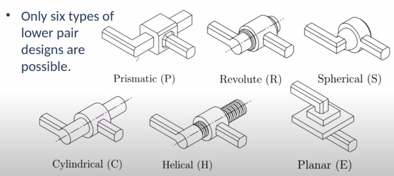
There are 6 types of lower pair joint designs possible.
- Revolute joint (R): This joint is like a hinge and allows for relative rotation between the two links. DOF = 1
- Prismatic joint (P): This joint allows for relative linear motion between the two links. DOF = 1
- Spherical joint (S): This joint allows for motion along all the three axes. DOF = 3
- Cylindrical joint (C): This joint allows for both rotation and linear motion between the two links. DOF = 2
- Helical joint (H): This joint can be thought of as a screw-nut and allows for motion only along one axis. The linear and rotatory motions are not independent of each other. DOF = 1.
- Planar joint (E): This joint allows for motion between two planes. DOF = 3
Gruebler’s equation
\[M = 3L - 2J-3G\]- M = degree of freedom or Mobility
- L = number of links
- J = number of full joints (1 DOF)
- G = number of grounded links (G is always 1)
Transformations
A linear transformation is one that preserves the linear and scalar multiplication rules of vectors.
A projective transformation shows how an object is perceived as the observer’s viewpoint changes.
An affine transformation is one that preserves collinearity (i.e., all points lying on a line continue to lie on the line after the transformation) and the ratio of distances between any 2 points on it remains the same. They are used for scaling, skewing and rotation.
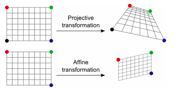
Source: https://www.graphicsmill.com/docs/gm/affine-and-projective-transformations.htm
Rigid transformations, also called Euclidean transformation, is one that preserves the Euclidean distance between every pair of points. It includes rotations, translations, reflections, or their combination. Scaling and shear are excluded from such a type of transformation. Sometimes reflections are also excluded by imposing that the transformation also preserves the handedness of figures.
Rotational Transformations
A transformation matrix called the Rotation Matrix is used to specify the coordinate vectors for the axes of a frame $o_1x_1y_1z_1$ *with respect to coordinate frame $o_0x_0y_0z_0$.* Thus, $R_1^0$ is a rotation matrix whose column vectors are the coordinates of the axes of frame $o_1x_1y_1z_1$ *expressed relative to coordinate frame $o_0x_0y_0z_0$.*
\[R_1^0 = \begin{bmatrix}x_1.x_0 & y_1.x_0 & z_1.x_0\\x_1.y_0 & y_1.y_0 & z_1.y_0\\x_1.z_0 & y_1.z_0 & z_1.z_0\end{bmatrix}\]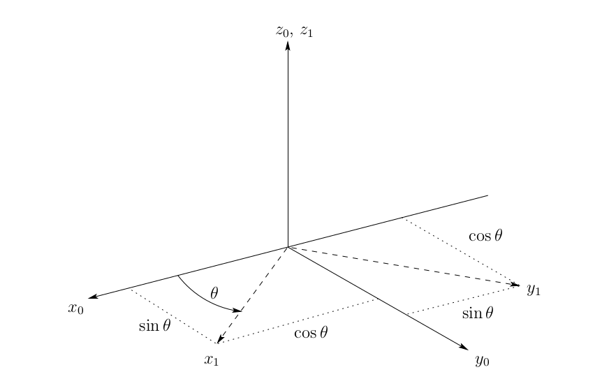
For a positive rotation about the z-axis by an angle θ, we have
\[x_1.x_0=cosθ\] \[x_1.y_0=sinθ\] \[y_1.x_0=-sinθ\] \[y_1.y_0=cosθ\] \[z_1.z_0=1\]Thus the rotation matrix equals
\[R_1^0=\begin{bmatrix} cosθ & -sinθ & 0\\sinθ & cosθ & 0\\ 0 & 0 & 1\end{bmatrix}\]If we wish to describe the orientation of frame $o_0x_0y_0z_0$ with respect to frame $o_1x_1y_1z_1$, we would have $R_0^1$ such that
\[R_0^1 = (R_1^0)^T = (R_1^0)^{-1}\]The rotation matrix $R_1^0$ can not only be used to represent the orientation of the coordinate frame $o_1x_1y_1z_1$ with respect to frame $o_0x_0y_0z_0$, but also to transform the coordinates of a point from one frame to the other. Thus if a given point is expressed with respect to the frame $o_1x_1y_1z_1$ as $p^1$then $R_1^0p^1$ represents the same point with respect to frame $o_0x_0y_0z_0$.
\[p^0=R_1^0p^1\]Instead of relating the coordinates of a fixed vector with respect to two different coordinate frames, the rotation matrix is also used to represent the coordinates of a vector $v_1$ obtained from a vector $v$ by a given rotation in the same coordinate frame.
Composition of Rotations
Rotation about current frame
In order to transform the coordinates of a point $p$ from its representation $p^2$ in the frame $o_2x_2y_2z_2$ to its representation $p^0$ in the frame $o_0x_0y_0z_0$ , we may first transform to its coordinates $p^1$ in the frame $o_1x_1y_1z_1$ using $R_2^1$ and then transform $p^1$ to $p^0$ using $R_1^0$. Thus,
\[R_2^0=R_1^0R_2^1\]Rotation about fixed frame
If we wish to perform successive rotations with respect to a fixed frame $o_0x_0y_0z_0$ instead of the current frame, then the above equation does not hold true anymore. Rather we need to multiply the rotation matrices in the reverse order.
Let $o_0x_0y_0z_0$ be the reference frame. Let the frame $o_1x_1y_1z_1$ be obtained by performing a rotation with respect to the reference frame, and let this rotation be denoted by $R_1^0$. Now let $o_2x_2y_2z_2$ be obtained by performing a rotation of frame $o_1x_1y_1z_1$ with respect to the reference frame (not with respect to frame $o_1x_1y_1z_1$ itself). Let this rotation be denoted by the matrix $R$. Let $R_2^0$ be the matrix that denotes the orientation of frame $o_2x_2y_2z_2$ w.r.t frame $o_0x_0y_0z_0$. Now
\[R_2^0 ≠ R_1^0R\]Instead,
\[R_2^0=RR_1^0\]Derivation:
We will convert the rotation about the fixed frame into one about the current frame. First we will rotate the frame $o_1x_1y_1z_1$ w.r.t the frame $o_0x_0y_0z_0$. This can be done by postmultiplying with the inverse of $R_1^0$. Now since the current frame is aligned with the reference frame, we can simply postmultiply with $R$ to get the frame $o_2x_2y_2z_2$. We now need to undo the initial rotation by postmultiplying with $R_1^0$. Therefore, we have
\[R_2^0=R_1^0R_2^1\\R_2^0=R_1^0[(R_1^0)^{-1}RR_1^0]\\R_2^0=RR_1^0\]Euler Angles
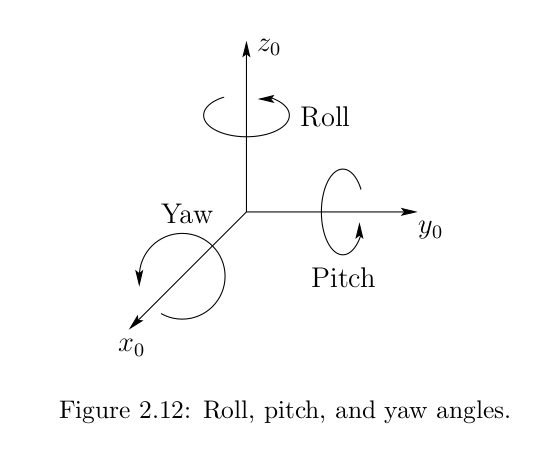
Roll, Pitch and Yaw Angles
A rotation by $\phi$ about $z_0$ is the roll angle, a rotation by $\theta$ about $y_0$ is the pitch angle, and a rotation by $\psi$ about $x_0$ is the yaw angle.
For the rotations yaw-pitch-roll w.r.t a fixed frame or for the rotations roll-pitch-yaw w.r.t current frame, we get the following transformation matrix
\[R_1^0=R_{z,\phi}R_{y,\theta}R_{x,\psi}\\=\begin{bmatrix}c_\phi & -s_\phi & 0\\s_\phi & c_\phi & 0\\0&0&1 \end{bmatrix}\begin{bmatrix}c_\theta& 0&s_\theta\\0&1&0\\-s_\theta&0&c_\theta\end{bmatrix}\begin{bmatrix}1&0&0\\0&c_\psi&-s_\psi\\0&s_\psi&c_\psi\end{bmatrix}\\\] \[=\begin{bmatrix}c_\phi c_\theta&-s_\phi c_\psi+c_\phi s_\theta s_\psi&s_\phi s_\psi+c_\phi s_\theta c_\psi\\s_\phi c_\theta&c_\phi c_\psi+s_\phi s_\theta s_\psi & -c_\phi s_\psi + s_\phi s_\theta c_\psi \\ -s_\theta&c_\theta s_\psi&c_\theta c_\psi\end{bmatrix}\]Homogeneous Transformations
If frame $o_1x_1y_1z_1$ is obtained from frame $o_0x_0y_0z_0$ by first applying a rotation specified by $R_1^0$ followed by a translation given (with respect to $o_0x_0y_0z_0$) by $d_1^0$ , then the coordinates $p^0$ are given by
\[p^0=R_1^0p^1+d_1^0\]In general,
\[r_p^G=R_B^Gr_p^B+d^G\]where $d^G$ is the displacement or translation of B w.r.t G.
If we have 2 rigid motions,
\[First \space motion: p^0=R_1^0p^1+d_1^0\] \[Second \space motion: p^1=R_2^1p^2+d_2^1\]On combining the two, we get
\[p^0=R_1^0(R_2^1p^2+d_2^1)+d_1^0 \\ p^0=R_1^0R_2^1p^2+d_1^0+R_1^0d_2^1\]This can also be expressed as
\[p^0=R_2^0p^2+d_2^0\]where
\[R_2^0=R_1^0R_2^1\\d_2^0=d_1^0+R_1^0d_2^1\] \[\begin{bmatrix}R_1^0&d_1^0\\0&1\end{bmatrix}\begin{bmatrix}R_2^1&d_2^1\\0&1\end{bmatrix}=\begin{bmatrix}R_1^0R_2^1&d_1^0+R_1^0d_2^1\\0&1\end{bmatrix}\] \[T_B^G=\begin{bmatrix}R_B^G&d^G\\0&1\end{bmatrix}\] \[T_G^B=\begin{bmatrix}R_B^G&d^G\\0&1\end{bmatrix}^{-1}=\begin{bmatrix}{R_B^G}^T&-{R_B^G}^Td^G\\0&1\end{bmatrix}\]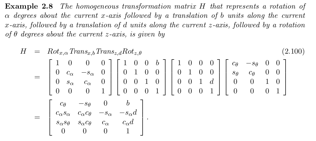
Forward Kinematics
In Forward Kinematics, we are to determine the position and orientation of the end-effector given the values for the joint variables of the robot. The joint variables are the angles between the links in the case of revolute or rotational joints, and the link extension in the case of prismatic or sliding joints.
The following conventions are defined to perform kinematic analysis:
- A robot manipulator with n joints will have n+1 links, since each joint connects to two links.
- Joints are numbered from 1 to n.
- Links are numbered from 0 to n, starting from the base.
- Joint i connects link i-1 to link i.
- When joint i is actuated, link i moves.
- A coordinate from $o_ix_iy_iz_i$ is rigidly attached to link i. So when a joint i moves, link i and its attached coordinate frame also moves.
Let $A_i$ be a homogeneous transformation matrix that expresses the position and orientation of frame $o_ix_iy_iz_i$ w.r.t frame $o_{i-1}x_{i-1}y_{i-1}z_{i-1}$.
$T_j^i$ is the transformation matrix that expresses the position and orientation of frame $o_jx_jy_jz_j$ w.r.t frame $o_ix_iy_iz_i$.
\[T_j^i=A_{i+1}A_{i+2}...A_{j-1}A_j \space \space if \space i<j\] \[T_j^i=I \space \space if\space i=j \\ T_j^i = (T_i^j)^{-1} \space if \space j>i\]Denavit-Hartenberg Convention
The following steps need to be followed to derive the forward kinematics for a manipulator:
Step 1: Locate and label the joint axes $z_0,z_1,…,z_{n-1}$. We assign $z_i$ to be the axis of actuation for joint $i+1$.
Step 2: Choose the base coordinate frame. Set the origin anywhere on the $z_0$ axis.
Step 3: Locate the origin $o_i$ where the common normal to $z_i$ and $z_{i-1}$ intersects $z_i$. If $z_i$ intersects $z_{i-1}$, $o_i$ is located at the point of intersection. If $z_i$ and $z_{i-1}$ are parallel, locate $o_i$ in any point along $z_i$.
Step 4: The x-axis is defined along the common normal between $z_{i-1}$ and $z_i$ axes through $o_i$, pointing from $z_{i-1}$ to $z_i$ axis. When the two axes are intersecting, $x_i$ is in the direction of $z_{i-1}$x $z_i$.
Step 5: Define $y_i$ to complete the right hand coordinate system.
Step 6: Choose $o_nx_ny_nz_n$ to be the end-effector frame.
Step 7: Create a table of the following parameters $a_i,d_i,\alpha_i,\theta_i$.
- Link length $a_i$: distance between $z_i$ and $z_{i-1}$axes along the $x_i$ axis.
- Joint distance $d_i$: distance between $x_{i-1}$ and $x_i$ axes along the $z_{i-1}$ axis.
- Link twist $\alpha_i$: required rotation of $z_{i-1}$ axis about the $x_i$ axis to become parallel to $z_i$ axis.
- Joint angle $\theta_i$: required rotation of $x_{i-1}$ axis about the $z_{i-1}$ axis to become parallel to $x_i$ axis.
Step 8: Form the homogeneous transformation matrix $A_i$ by substituting the above parameters.
\[A_i=Rot_{z,\theta_i}Trans_{z,d_i}Trans_{x,a_i}Rot_{x,\alpha_i} \\ = \begin{bmatrix} c_{\theta_i} & -s_{\theta_i}c_{\alpha_i} & s_{\theta_i}s_{\alpha_i} & a_ic_{\theta_i} \\ s_{\theta_i} & c_{\theta_i}c_{\alpha_i} & -c_{\theta_i}s_{\alpha_i} & a_is_{\theta_i}\\0&s_{\alpha_i}&c_{\alpha_i}&d_i\\0&0&0&1 \end{bmatrix}\]Step 9: Form the transformation matrix $T_n^0=A_1A_2…A_n$. This gives the position and orientation of the end-effector w.r.t the base frame.
Stanford Manipulator:
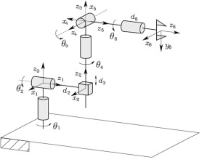
DH-parameters:
| Link | ⁍ | ⁍ | ⁍ | ⁍ |
|---|---|---|---|---|
| 1 | 0 | 0 | -90 | * |
| 2 | ⁍ | 0 | 90 | * |
| 3 | * | 0 | 0 | 0 |
| 4 | 0 | 0 | -90 | * |
| 5 | 0 | 0 | 90 | * |
| 6 | ⁍ | 0 | 0 | * |
We can plug in the above values into the $A_i$ matrix to get $A_1,A_2,A_3,A_4,A_5,A_6$. This gives us $T_6^0 = A_1A_2…A_6.$
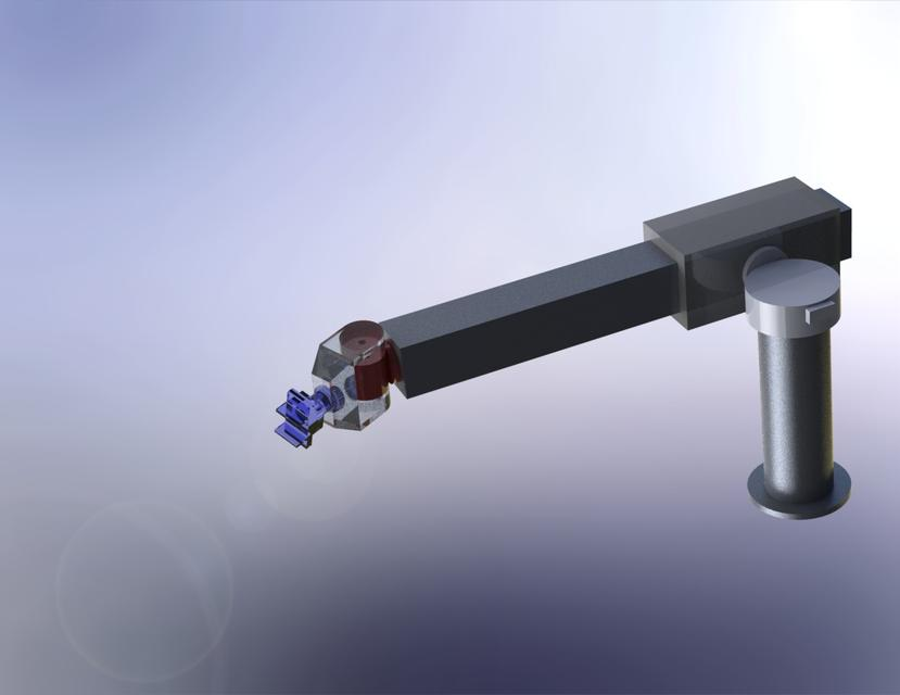
SCARA Manipulator
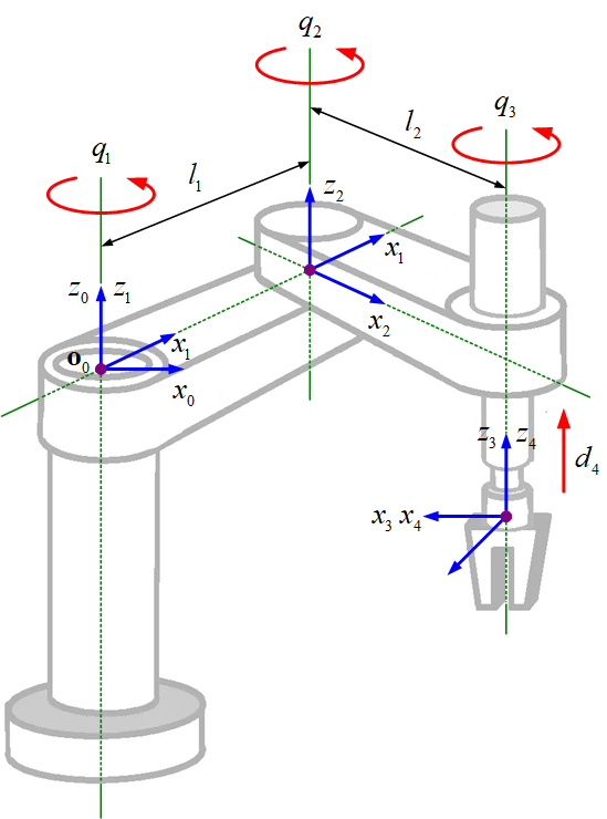
Has 4 DOF - 3R+1P
DH-parameters:
| Link | ⁍ | ⁍ | ⁍ | ⁍ |
|---|---|---|---|---|
| 1 | 0 | 0 | 0 | * |
| 2 | 0 | ⁍ | 0 | * |
| 3 | ⁍ | ⁍ | 0 | 0 |
| 4 | 0 | 0 | 0 | * |
Reference: https://www.youtube.com/watch?v=O8nzaDcjTiY