
Introduction
The following project shows the implementation of a simple convolutional neural network (CNN). The model will be able to identify which signal it is when presented with a colour image of a traffic sign. Being my first project in deep learning, I gained extensive knowledge about how the dataset is composed, how to pre-process images, which deep network to use, and how to efficiently choose the number of layers and units.
Dataset
The dataset used for this project can be obtained from Public Archive: daaeac0d7ce1152aea9b61d9f1e19370
Data Preprocessing
The entire dataset contains images of different sizes. Since the very first operation of the model involves reading and standardizing the images, it is important to resize all the images to a predefined size, 32x32 in this case. The colorspace of the images is also converted from RGB to grayscale.
Another important data preprocessing step is one-hot encoding. One-hot encoding refers to the process of converting categorical data variables to a numerical form, and this is done with a 43-dimensional array.
Image Resizing
1
2
3
4
5
6
7
8
9
10
11
12
13
14
15
16
17
18
19
20
21
22
23
24
25
26
27
28
29
30
31
32
33
34
35
36
37
38
39
40
import numpy as np
import matplotlib.pyplot as plt
from skimage.color import rgb2lab
from skimage.transform import resize
import glob
from collections import namedtuple
%matplotlib inline

N_CLASSES = 43
RESIZED_IMAGE = (32,32)

Dataset = namedtuple('Dataset',['X','y'])

def read_dataset_ppm(rootpath, n_labels, resize_to):
    images = []
    labels = []

    for c in range(n_labels):
        full_path = rootpath + '/' + format(c,'05d') + '/'

        for img_name in glob.glob(full_path + '*.ppm'):
            img = plt.imread(img_name).astype(np.float32)
            img = rgb2lab(img/255.0)[:,:,0]

            img = resize(img, resize_to, mode='reflect').astype(np.float32)

            label = np.zeros(shape=(n_labels,), dtype=np.float32)
            label[c] = 1.0
            labels.append(label)
            images.append(img)

    return Dataset(X = img_stack(/assets/images/L3D/a3/images), y = np.array(labels))

def img_stack(imgs):
    return np.stack([img[:,:,np.newaxis] for img in imgs], axis=0).astype(np.float32)

dataset = read_dataset_ppm('GTSRB_Final_Training_Images/GTSRB/Final_Training/Images', N_CLASSES, RESIZED_IMAGE)

print(dataset.X.shape)
print(dataset.y.shape)
Train test split
1
2
3
4
5
6
7
8
from sklearn.model_selection import train_test_split

idx_train, idx_test = train_test_split(range(dataset.X.shape[0]), test_size=0.25)

X_train = dataset.X[idx_train,:,:]
X_test = dataset.X[idx_test,:,:]
y_train = dataset.y[idx_train,:]
y_test = dataset.y[idx_test,:]
Creating minibatches of data
Every training iteration would require the addition of a minibatch of randomly chosen samples taken from the practise set. Different minibatches of data in every generator will compel the model to learn the in-out connection rather than memorizing the sequence.
1
2
3
4
5
6
7
8
9
10
11
n_samples = X_train.shape[0]

def minibatcher(X, y, batch_size):

    i = np.random.permutation(n_samples)

    for j in range(int(np.ceil(n_samples/batch_size))):
        fr = j * batch_size
        to = (j+1) * batch_size

        yield X[i[fr:to],:,:,:], y[i[fr:to],:]
Layers
1
2
3
4
5
6
7
8
9
10
11
12
13
14
15
16
17
18
19
20
21
22
23
24
25
26
27
28
29
30
31
32
33
34
35
36
37
import tensorflow.compat.v1 as tf
tf.disable_v2_behavior()

def fc_no_activation(in_tensors, n_units):
    w = tf.get_variable(name="fc_W",
                        shape=[in_tensors.get_shape()[1], n_units],
                       dtype=tf.float32,
                       initializer=tf.keras.initializers.glorot_normal())
    b = tf.get_variable(name="fc_B",
                        shape=[n_units,],
                       dtype=tf.float32,
                       initializer=tf.constant_initializer(0.0))
    return tf.matmul(in_tensors,w) + b

# Fully connected layer
def fc_layer(in_tensors, n_units):
    return tf.nn.leaky_relu(fc_no_activation(in_tensors, n_units))

# COnvolution layer
def conv_layer(in_tensors, kernel_size, n_units):
    w = tf.get_variable(name="conv_W",
                        shape=[kernel_size, kernel_size, in_tensors.get_shape()[3], n_units],
                       dtype=tf.float32,
                       initializer=tf.keras.initializers.glorot_normal())
    b = tf.get_variable(name="conv_B",
                        shape=[n_units,],
                       dtype=tf.float32,
                       initializer=tf.constant_initializer(0.0))
    return tf.nn.leaky_relu(tf.nn.conv2d(input=in_tensors, filters=w, strides=[1,1,1,1], padding='SAME') + b)

# Maxpool layer
def maxpool_layer(in_tensors, sampling):
    return tf.nn.max_pool(in_tensors, [1, sampling, sampling, 1], [1, sampling, sampling, 1], 'SAME')

# Dropout layer
def dropout(in_tensors, keep_proba, is_training):
    return tf.cond(is_training, lambda: tf.nn.dropout(in_tensors, keep_proba), lambda: in_tensors)
Structure
The model will be composed of the following layers:
- 2D convolution, 5x5, 32 filters
- 2D convolution, 5x5, 64 filters
- Flattenizer
- Fully connected later, 1,024 units
- Dropout 40%
- Fully connected layer, no activation
- Softmax output
1
2
3
4
5
6
7
8
9
10
11
12
13
14
15
16
17
18
19
20
21
22
23
24
25
26
27
def model(in_tensors, is_training):

    # First layer: 5x5 2d-conv, 32 filters, 2x maxpool, 20% drouput
    with tf.variable_scope('l1', reuse=tf.AUTO_REUSE):
        l1_conv = conv_layer(in_tensors, 5, 32)
        l1_maxpool = maxpool_layer(l1_conv, 2)
        l1_drop = dropout(l1_maxpool, 0.8, is_training)

    # Second layer: 5x5 2d-conv, 64 filters, 2x maxpool, 20% drouput
    with tf.variable_scope('l2', reuse=tf.AUTO_REUSE):
        l2_conv = conv_layer(l1_drop, 5, 64)
        l2_maxpool = maxpool_layer(l2_conv, 2)
        l2_drop = dropout(l2_maxpool, 0.8, is_training)

    with tf.variable_scope('flatten', reuse=tf.AUTO_REUSE):
        l2_flatten = tf.layers.flatten(l2_drop)

    # Fully collected layer, 1024 neurons, 40% dropout
    with tf.variable_scope('l3', reuse=tf.AUTO_REUSE):
        l3 = fc_layer(l2_flatten, 1024)
        l3_drop = dropout(l3, 0.6, is_training)

    # OUTPUT
    with tf.variable_scope('output', reuse=tf.AUTO_REUSE):
        output_tensors = fc_no_activation(l3_drop, N_CLASSES)

    return output_tensors
Training
1
2
3
4
5
6
7
8
9
10
11
12
13
14
15
16
17
18
19
20
21
22
23
24
25
26
27
28
29
30
31
32
33
34
35
36
37
38
39
40
41
42
43
44
45
46
47
48
49
50
51
52
53
54
55
56
from sklearn.metrics import classification_report, confusion_matrix
def train_model(X_train, y_train, X_test, y_test, learning_rate, max_epochs, batch_size):
in_X_tensors_batch = tf.placeholder(tf.float32, shape=(None, RESIZED_IMAGE[0], RESIZED_IMAGE[1], 1))
in_y_tensors_batch = tf.placeholder(tf.float32, shape=(None, N_CLASSES))
is_training = tf.placeholder(tf.bool)
logits = model(in_X_tensors_batch, is_training)
out_y_pred = tf.nn.softmax(logits)
loss_score = tf.nn.softmax_cross_entropy_with_logits(logits=logits, labels=in_y_tensors_batch)
loss = tf.reduce_mean(loss_score)
optimizer = tf.train.AdamOptimizer(learning_rate).minimize(loss)
with tf.compat.v1.Session() as session:
session.run(tf.global_variables_initializer())
for epoch in range(max_epochs):
print("Epoch=", epoch)
tf_score = []
for mb in minibatcher(X_train, y_train, batch_size):
tf_output = session.run([optimizer, loss],
feed_dict={in_X_tensors_batch:mb[0],
in_y_tensors_batch:mb[1],
is_training:True})
tf_score.append(tf_output[1])
print("train_loss_score=",np.mean(tf_score))
print("TEST SET PERFORMANCE")
y_test_pred, test_loss = session.run([out_y_pred, loss],
feed_dict={in_X_tensors_batch:X_test,
in_y_tensors_batch:y_test,
is_training:False})
print(" test_loss_score=", test_loss)
# CLASSIFICATION REPORT
y_test_pred_classified = np.argmax(y_test_pred, axis=1).astype(np.int32)
y_test_true_classified = np.argmax(y_test, axis=1).astype(np.int32)
print(classification_report(y_test_true_classified, y_test_pred_classified))
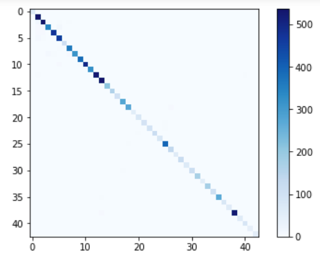
# CONFUSION MATRIX
cm = confusion_matrix(y_test_true_classified, y_test_pred_classified)
plt.imshow(cm, interpolation='nearest', cmap=plt.cm.Blues)
plt.colorbar()
plt.tight_layout()
plt.show()
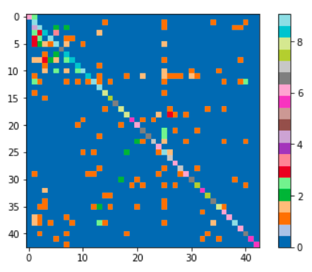
# And the log2 version, to enphasize the misclassifications
plt.imshow(np.log2(cm + 1), interpolation='nearest', cmap=plt.get_cmap("tab20"))
plt.colorbar()
plt.tight_layout()
plt.show()
tf.reset_default_graph()
train_model(X_train, y_train, X_test, y_test, 0.001, 10, 256)
Results
Accuracy = 98%
Performance Report
1
2
3
4
5
6
7
8
9
10
11
12
13
14
15
16
17
18
19
20
21
22
23
24
25
26
27
28
29
30
31
32
33
34
35
36
37
38
39
40
41
42
43
44
45
46
47
48
49
50
51
52
53
54
55
56
57
58
59
60
61
62
63
64
65
66
67
68
69
70
71
Epoch= 0
train_loss_score= 4.8711586
Epoch= 1
train_loss_score= 0.83951813
Epoch= 2
train_loss_score= 0.3692537
Epoch= 3
train_loss_score= 0.2198893
Epoch= 4
train_loss_score= 0.1685863
Epoch= 5
train_loss_score= 0.11884567
Epoch= 6
train_loss_score= 0.10304754
Epoch= 7
train_loss_score= 0.07655481
Epoch= 8
train_loss_score= 0.072380714
Epoch= 9
train_loss_score= 0.059970096
TEST SET PERFORMANCE
 test_loss_score= 0.0674421
              precision    recall  f1-score   support

           0       1.00      1.00      1.00        45
           1       0.99      0.98      0.98       545
           2       0.92      1.00      0.96       561
           3       0.99      0.98      0.99       357
           4       0.98      0.98      0.98       484
           5       0.99      0.94      0.97       472
           6       1.00      1.00      1.00       104
           7       1.00      0.97      0.98       347
           8       1.00      0.97      0.98       372
           9       0.99      0.99      0.99       370
          10       0.99      1.00      1.00       500
          11       1.00      0.97      0.99       352
          12       0.99      1.00      0.99       538
          13       1.00      0.99      1.00       549
          14       0.99      1.00      0.99       193
          15       0.99      0.99      0.99       166
          16       0.99      0.99      0.99        96
          17       1.00      0.99      1.00       293
          18       0.97      1.00      0.99       276
          19       1.00      0.98      0.99        44
          20       0.95      0.99      0.97        93
          21       0.96      0.99      0.97        77
          22       0.99      1.00      1.00       119
          23       0.97      0.98      0.98       127
          24       0.96      0.99      0.97        72
          25       0.98      0.98      0.98       396
          26       0.97      0.97      0.97       155
          27       1.00      1.00      1.00        68
          28       0.96      0.99      0.98       133
          29       0.98      0.89      0.93        64
          30       1.00      0.91      0.95       113
          31       1.00      0.98      0.99       195
          32       1.00      1.00      1.00        53
          33       1.00      0.96      0.98       170
          34       1.00      0.98      0.99        98
          35       1.00      1.00      1.00       263
          36       0.99      0.98      0.98        98
          37       1.00      1.00      1.00        48
          38       0.99      1.00      0.99       519
          39       1.00      1.00      1.00        64
          40       0.95      0.99      0.97        89
          41       1.00      0.98      0.99        61
          42       1.00      0.97      0.98        64

    accuracy                           0.98      9803
   macro avg       0.99      0.98      0.98      9803
weighted avg       0.99      0.98      0.98      9803
Confusion Matrix