Finite Markov Decision Process

A Finite Markov Decision Process (MDP) is a mathematical framework used to model sequential decision-making problems where an agent interacts with an environment over time. It is defined as a tuple $(S, A, p, r, \gamma)$, where each component captures one aspect of this interaction.

The state space $S$ is a finite set of all possible situations the agent can be in.
The action space $A$ is a finite set of choices available to the agent.
The transition function $p$ describes how the environment evolves: given the current state and action, it specifies the probability of transitioning to the next state.
The reward function $r$ assigns a scalar feedback signal that tells the agent how desirable a state–action pair is.
The discount factor $\gamma \in [0,1]$ controls how much the agent values future rewards relative to immediate ones.

Agent, Policy, Model, and Planning

An agent is the decision-making entity. It perceives the environment through sensors, acts through actuators, and has goals it wants to achieve. A policy is the agent’s behavior: it specifies what action to take in each state. Formally, a policy is a probability distribution over actions given states.

\[\pi(a \mid s) = \Pr(A_t = a \mid S_t = s), \forall t\]

A model describes how the environment works — it predicts the next state and reward given the current state and action. Planning means using this model to look ahead into the future and choose actions that achieve a goal. A plan is simply a sequence of actions. In reinforcement learning, the agent often does not know the model in advance and must learn through interaction.

The goal of reinforcement learning is to learn a policy. Policies are typically assumed to be stationary, meaning the same policy is used at every time step. During learning, the agent updates its policy based on experience.

Markovian States (Why History Can Be Thrown Away)

A state is called Markovian if it contains all the information needed to predict the future. This is known as the Markov property: given the current state and action, the future is independent of the past. Intuitively, this means the state is a sufficient summary of everything that has happened so far.

\[\Pr(R_{t+1}, S_{t+1} \mid S_0, A_0, \dots, S_t, A_t)=\Pr(R_{t+1}, S_{t+1} \mid S_t, A_t)\]

Rewards and Returns

Rewards are scalar signals provided by the environment that indicate progress toward a goal. Importantly, rewards define what the agent should accomplish, not how to do it. Almost all goal-directed behavior can be framed as maximizing the expected cumulative reward.

The reward function is often written as an expectation:

\[r(s, a) = \mathbb{E}[R_{t+1} \mid S_t = s, A_t = a]\]

In episodic tasks, interaction naturally breaks into episodes with a clear end, such as a game or navigating a maze. The return is the total reward accumulated until the terminal state:

\[G_t = R_{t+1} + R_{t+2} + \dots + R_T\]

Here, $T$ is the final time step of the episode. The agent’s objective is to maximize this return.

In continuing tasks, there is no natural episode boundary (e.g., robot control or stock trading). In this case, we use discounted returns to ensure the total reward remains finite and to prioritize near-term outcomes:

\[G_t = R_{t+1} + \gamma R_{t+2} + \gamma^2 R_{t+3} + \dots = \sum_{k=0}^\infty \gamma^k R_{t+k+1}\]

The discount factor $\gamma$ determines how farsighted the agent is.

Value-Based vs Policy-Based Reinforcement Learning

Value-based methods focus on learning a value function: a function that tells us how good a state or state-action pair is in terms of expected future reward. Once this value function is learned, the policy is not learned explicitly; instead, it is implicit, typically derived by choosing the action with the highest value (for example, using $\epsilon-$greedy exploration). Algorithms like Q-learning fall into this category.

Policy-based methods flip this idea around. Instead of learning values and deriving actions from them, the agent directly learns the policy itself, which is a mapping from states to actions or action distributions. There is no requirement to maintain or estimate a value function. The policy parameters are adjusted so that actions sampled from the policy lead to higher long-term reward. This makes policy-based methods especially natural for continuous action spaces, where choosing an action by “argmax over values” is awkward or ill-defined.

Actor-Critic methods sit exactly at the intersection of these two ideas. They learn both a policy (the actor) and a value function (the critic). The critic evaluates how good the actor’s actions are, and this feedback is used to update the policy more efficiently and with lower variance.

Policy-Based RL

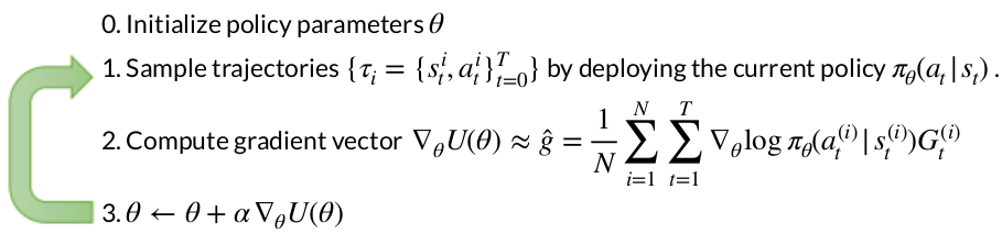
Policy-based reinforcement learning can be cleanly framed as a direct optimization problem. We define an objective function $U(\theta)$, which measures how good a policy parameterized by $\theta$ is. This is typically the expected cumulative reward when following that policy.

Learning then proceeds by iteratively improving the policy parameters. At each iteration, we first roll out the current policy in the environment to collect trajectories (sequences of states and actions generated by following the policy). Using these trajectories, we estimate how changing the policy parameters would affect the objective. Finally, we update the parameters in the direction that increases the objective. Intuitively, this is just like standard gradient ascent.

\[\theta_{\text{new}} = \theta_{\text{old}} + \alpha \nabla_\theta U(\theta)\]

Why are they useful?

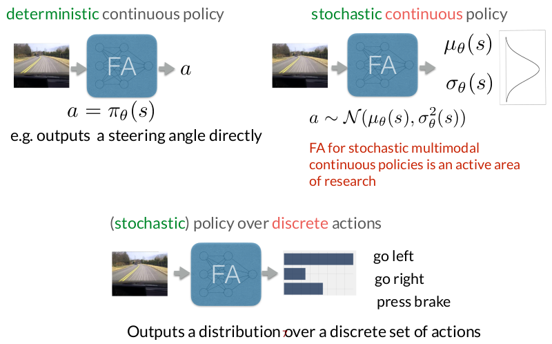
One major advantage of policy-based methods is that they handle high-dimensional and continuous action spaces naturally. Instead of evaluating many possible actions and selecting the best one, the policy directly outputs an action (or a distribution over actions). This is especially important in robotics, where actions are often continuous (e.g., torques, velocities, steering angles).

Another key benefit is the ability to learn stochastic policies. Rather than committing to a single action in each state, the policy can represent uncertainty or intentional randomness, which is often crucial for exploration or for modeling multimodal behaviors.

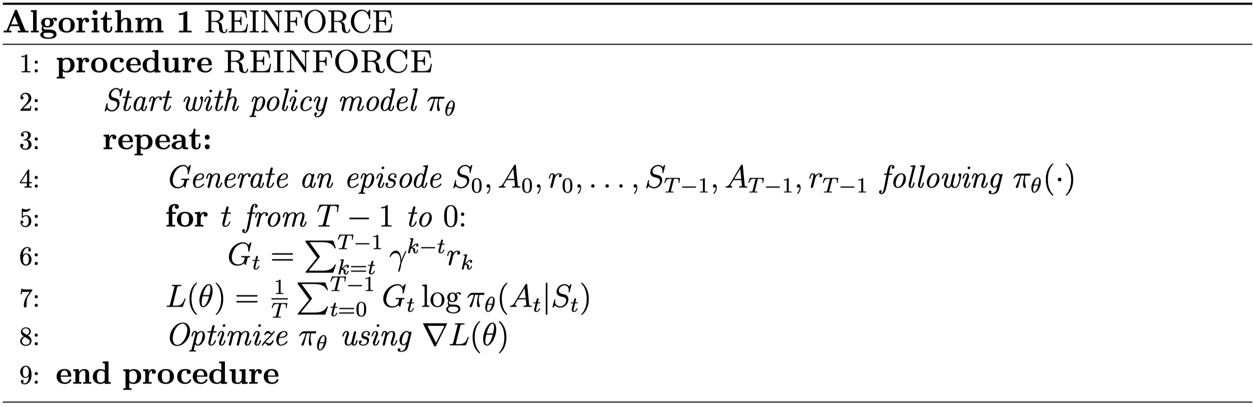
REINFORCE (or Monte Carlo Policy Gradient)

In policy-based reinforcement learning, the agent does not try to estimate values first and then derive a policy. Instead, it directly optimizes the policy itself. To do this, we need to define a clear objective that tells us how good a policy is.

A trajectory $\tau$ is one full rollout of the agent interacting with the environment. It is simply a sequence of states and actions:

\[\tau = (s_0, a_0, s_1, a_1, \dots, s_H, a_H)\]

where $H$ is the horizon (episode length). Intuitively, a trajectory is “one attempt” by the agent to solve the task from start to finish.

Since the environment is stochastic (and the policy may be stochastic too), the agent does not experience the same trajectory every time. Instead, trajectories are sampled from a probability distribution induced by the policy. Therefore, a reasonable objective is to maximize the expected trajectory reward:

Intuition: “On average, how much reward does my policy get when I deploy it in the environment?”

The expectation can also be written explicitly as a sum over all possible trajectories:

\[U(\theta) = \sum_{\tau} P(\tau; \theta)\, R(\tau)\]

Probability of a Trajectory:

A trajectory is generated by two components:

Environment dynamics: how states evolve
Policy: how actions are chosen

The probability of a trajectory factorizes as:

The dynamics term $P(s_{t+1} \mid s_t,a_t)$ is fixed and unknown
The policy term $\pi_{\theta}(a_t \mid s_t)$ is what we control and parameterize

Derivation

Our goal is not to compute the objective itself, but to compute its gradient with respect to the policy parameters:

\[\nabla_\theta U(\theta)= \nabla_\theta \mathbb{E}_{\tau \sim P(\tau; \theta)}[R(\tau)]\] \[\nabla_\theta U(\theta)= \sum_{\tau} \nabla_\theta P(\tau; \theta)\, R(\tau)\]

Now apply the log-derivative trick:

\[\nabla_\theta P(\tau; \theta)= P(\tau; \theta)\, \nabla_\theta \log P(\tau; \theta)\]

Substitute:

\[\nabla_\theta U(\theta)= \sum_{\tau} P(\tau; \theta)\, \nabla_\theta \log P(\tau; \theta)\, R(\tau)\]

This can be written as an expectation:

\[\nabla_\theta U(\theta)= \mathbb{E}_{\tau \sim P(\tau; \theta)}\left[ \nabla_\theta \log P(\tau; \theta)\, R(\tau) \right]\]

Recall the trajectory probability:

\[\log P(\tau; \theta)= \sum_{t=0}^{H} \log P(s_{t+1} \mid s_t, a_t)+ \sum_{t=0}^{H} \log \pi_\theta(a_t \mid s_t)\]

The environment dynamics do not depend on $\theta$, so their gradient is zero. This leaves:

\[\nabla_\theta \log P(\tau; \theta)= \sum_{t=0}^{H} \nabla_\theta \log \pi_\theta(a_t \mid s_t)\]

Substitute back into the gradient:

Using Monte-Carlo sampling with $N$ trajectories:

Intuition:

Each term $\nabla_\theta \log \pi_\theta(a_t^{(i)}\mid s_t^{(i)})$ asks: “How should I change the policy parameters to make this action more likely in this state?”

That change is scaled by the total reward $R(\tau)$:

If the trajectory was good $\rightarrow$ reinforce the actions
If the trajectory was bad $\rightarrow$ suppress the actions

So learning boils down to: Increase the probability of actions that led to good outcomes, decrease the probability of actions that led to bad ones.

Assigning the full trajectory return to every action is wasteful. An action at time $t$ cannot affect rewards that happened before it. So we define the return from time $t$ onward:

\[G_t = \sum_{k=t}^{H} R(s_k, a_k)\]

Replace $R(\tau)$ with $G_t$:

Gaussian Policy

Assume a continuous action space. The policy outputs the parameters of a Gaussian:

\[\pi_\theta(a \mid s) = \mathcal{N}\big(a \mid \mu_\theta(s), \sigma^2\big)\]

To keep things simple:

Mean $\mu_\theta(s)$ depends on $\theta$
Variance $\sigma^2$ is fixed

So at state $s_t$:

The network outputs $\mu_\theta(s_t)$
The action is sampled:
\[a_t \sim \mathcal{N}(\mu_\theta(s_t), \sigma^2)\]

For a 1D Gaussian:

\[\log \pi_\theta(a_t \mid s_t)= -\frac{1}{2\sigma^2}(a_t - \mu_\theta(s_t))^2 + C\]

We ignore constants because they vanish under gradients.

\[\nabla_\theta \log \pi_\theta(a_t \mid s_t)= \frac{(a_t - \mu_\theta(s_t))}{\sigma^2}\nabla_\theta \mu_\theta(s_t)\]

For a 2D Gaussian:

The policy outputs a mean vector:

\[\mu_\theta(s)=\begin{bmatrix}\mu_1(s) \\\mu_2(s)\end{bmatrix}\]

We assume a Gaussian policy with fixed covariance:

\[\pi_\theta(a \mid s)=\mathcal{N}\big(a \mid \mu_\theta(s), \Sigma\big)\] \[a \sim \mathcal{N}(\mu_\theta(s), \Sigma)\] \[\log \pi_\theta(a \mid s)=-\frac{1}{2}(a - \mu_\theta(s))^\top\Sigma^{-1}(a - \mu_\theta(s))+ C\] \[\nabla_\theta \log \pi_\theta(a \mid s)=\Sigma^{-1}(a - \mu_\theta(s))\;\nabla_\theta \mu_\theta(s)\]

This is the multi-dimensional generalization of the 1D case.

Geometric Intuition:

The vector $(a - \mu_\theta(s))$ points from the mean to the sampled action.

Then:

$\Sigma^{-1}$ scales that vector
Directions with low variance get amplified
Directions with high variance get damped

So the gradient says: “Move the mean toward the sampled action, but trust directions where the policy is more confident.”

REINFORCE Update in 2D:

\[\Delta \theta\propto\Sigma^{-1}(a_t - \mu_\theta(s_t))\nabla_\theta \mu_\theta(s_t)\; G_t\]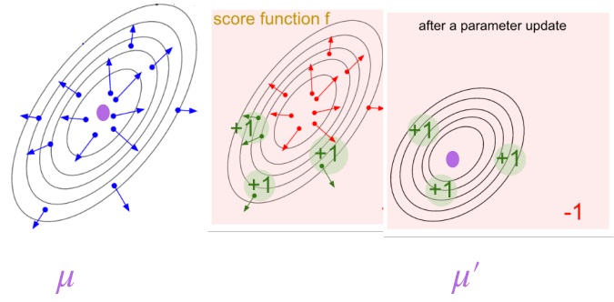

Softmax Policy

Now assume the action space is discrete. Instead of outputting a mean and variance, the policy outputs a score (logit) for each action. Let this score function be $h_\theta(s,a)$.

The policy converts scores into probabilities using softmax:

\[\pi_\theta(a \mid s)=\frac{\exp(h_\theta(s, a))}{\sum_{b} \exp(h_\theta(s, b))}\]

Key idea:

Higher score $\rightarrow$ higher probability
Scores are unconstrained real numbers
Softmax turns them into a valid probability distribution

\[\log \pi_\theta(a \mid s)=h_\theta(s, a)-\log \sum_{b} \exp(h_\theta(s, b))\] \[\nabla_\theta \log \pi_\theta(a \mid s) = \nabla_\theta h_\theta(s,a) - \nabla_\theta \log \sum_{b} \exp(h_\theta(s,b))\] \[\nabla_\theta \log \sum_{b} \exp(h_\theta(s,b))=\frac{1}{\sum_{b} \exp(h_\theta(s,b))}\nabla_\theta \sum_{b} \exp(h_\theta(s,b))\] \[\nabla_\theta \sum_{b} \exp(h_\theta(s,b))=\sum_{b} \nabla_\theta \exp(h_\theta(s,b)) =\sum_{b} \exp(h_\theta(s,b)) \nabla_\theta h_\theta(s,b)\] \[\nabla_\theta \log \sum_{b} \exp(h_\theta(s,b))=\frac{\sum_{b} \exp(h_\theta(s,b)) \nabla_\theta h_\theta(s,b)}{\sum_{b} \exp(h_\theta(s,b))} \\ = \sum_{b} \frac{\exp(h_\theta(s,b))}{\sum_{b'} \exp(h_\theta(s,b'))} \nabla_\theta h_\theta(s,b)\]

But this fraction is exactly the softmax probability:

\[\pi_\theta(b \mid s)=\frac{\exp(h_\theta(s,b))}{\sum_{b'} \exp(h_\theta(s,b'))}\]

So the entire term becomes:

\[\nabla_\theta \log \sum_{b} \exp(h_\theta(s,b))=\sum_{b} \pi_\theta(b \mid s)\, \nabla_\theta h_\theta(s,b)\] \[\nabla_\theta \log \pi_\theta(a \mid s)=\nabla_\theta h_\theta(s,a)-\sum_{b} \pi_\theta(b \mid s)\, \nabla_\theta h_\theta(s,b)\]

Intuition:

The softmax policy gradient has two terms because learning in discrete action spaces is about redistributing probability mass, not independently increasing action scores. Increasing the score of a chosen action must be balanced by decreasing the scores of other actions to preserve normalization. The gradient therefore increases the score of the selected action while subtracting the probability-weighted average score gradient of all actions, ensuring that probability mass shifts toward better actions in a competitive manner.

Algorithm:

Limitations

Mathematically, the REINFORCE update is:

\[\nabla_\theta U(\theta)\approx\sum_{t}\nabla_\theta \log \pi_\theta(a_t \mid s_t)\, G_t\]

The return $G_t$ is a very blunt learning signal. It mixes together two fundamentally different effects:

State quality: some states are inherently good or bad
Action quality: some actions are better than others within the same state

REINFORCE cannot distinguish between these. If the agent is in a bad state, all actions receive low returns and are suppressed, even if one of them was the best possible choice. Conversely, in a good state, all actions are reinforced, even if some were poor.

This is why REINFORCE updates are extremely noisy: it is trying to solve a fine-grained credit assignment problem using a coarse, trajectory-level signal.

Actor-Critic

Building upon the limitations of the REINFORCE algorithm, we infer a key conceptual insight: we should not judge an action by how good the episode was, but by how good the action was relative to the state in which it was taken.

Baseline

REINFORCE updates the policy using returns:

\[\nabla_\theta U(\theta)\approx\sum_t\nabla_\theta \log \pi_\theta(a_t \mid s_t)\, G_t\]

This estimator is unbiased, but extremely high variance. This is because the return $G_t$ contains a lot of irrelevant information. It depends on:

the quality of the state
randomness in the environment
future actions that had nothing to do with the current action

So the policy gradient ends up reacting strongly to things the action did not cause. Intuitively, the algorithm is asking “Was this episode good?”, when it should be asking “Was this action good for this state?”

If the agent is in a bad state, all actions receive low returns and are suppressed, even if one of them was the best possible choice. Conversely, in a good state, all actions are reinforced, even if some were poor. This is why REINFORCE updates are extremely noisy: it is trying to solve a fine-grained credit assignment problem using a coarse, trajectory-level signal.

The baseline exists to fix exactly this mismatch.

A baseline is simply a reference value that we subtract from the return before using it as a learning signal. So instead of using $G_t$, we use $(G_t-b)$.

Baseline choices:

Constant baseline (single scalar): $b = \mathbb{E}[R(\tau)]$
\[\hat{g}=\frac{1}{N}\sum_{i=1}^{N}\sum_{t=1}^{T}\nabla_\theta \log \pi_\theta(a_t^{(i)} \mid s_t^{(i)})\left(G_t^{(i)} - b\right)\]
This baseline removes global reward bias. If all trajectories tend to have large positive (or negative) returns, the policy gradient would otherwise push parameters strongly even when actions are not particularly informative. The constant baseline recenters the learning signal so that updates reflect relative success across trajectories.
Time-dependent Baseline (a vector length $T$): $b_t = \frac{1}{N} \sum_{i=1}^{N} G_t^{(i)}$
\[\hat{g}=\frac{1}{N}\sum_{i=1}^{N}\sum_{t=1}^{T}\nabla_\theta \log \pi_\theta(a_t^{(i)} \mid s_t^{(i)})\left(G_t^{(i)} - b_t\right)\]
Many tasks have systematic reward structure over time. Early actions tend to have larger remaining returns than late actions simply because more rewards are still ahead. A time-dependent baseline removes this predictable temporal effect, allowing the gradient to focus on deviations from the average behavior at that timestep.
State-dependent Baseline (a function):
\[b(s)=\mathbb{E}[r_t + r_{t+1} + \dots + r_{T-1} \mid s_t = s]=V^\pi(s)\] \[\hat{g}=\frac{1}{N}\sum_{i=1}^{N}\sum_{t=0}^{T}\nabla_\theta \log \pi_\theta(a_t^{(i)} \mid s_t^{(i)})\left(G_t^{(i)} - V^\pi(s_t^{(i)})\right)\]
Subtracting this baseline removes the effect of how easy or difficult the state is, leaving only information about the quality of the chosen action. The learning signal now answers a precise question: was this action better or worse than what I normally do in this state? This produces stable, low-variance updates and leads directly to the advantage function.

We want to encourage an action not when it has high return, but when it has higher return than the other actions from that state, that is, when it has an advantage over the other actions. It may well be that a state is bad and all actions have low returns in that state, but we do not care. The actions that have higher returns than the rest are the ones we want to reinforce. Therefore, we need to calibrate the goodness of actions using state-dependent baselines.

Why subtracting a baseline helps?

Consider two states:

A good state where all actions give high reward
A bad state where all actions give low reward

Without a baseline, good states reinforce everything, and bad states suppress everything. This is useless for learning which action is better.

With a baseline, only actions that outperform the state average are reinforced, and only actions that underperform are suppressed.

So the baseline removes the effect of state quality from the learning signal.

Does subtracting a baseline change the gradient?

The true policy gradient is:

\[\nabla_\theta U(\theta)=\mathbb{E}_{\tau \sim \pi_\theta}\left[\sum_t\nabla_\theta \log \pi_\theta(a_t \mid s_t)\, G_t\right]\]

Now suppose we subtract a baseline $b(s_t)$:

\[\mathbb{E}\left[\sum_t\nabla_\theta \log \pi_\theta(a_t \mid s_t)\,(G_t - b(s_t))\right]\] \[=\mathbb{E}\left[\sum_t\nabla_\theta \log \pi_\theta(a_t \mid s_t)\, G_t\right]-\mathbb{E}\left[\sum_t\nabla_\theta \log \pi_\theta(a_t \mid s_t)\, b(s_t)\right]\]

Focus on the second term:

\[\mathbb{E}\left[\nabla_\theta \log \pi_\theta(a_t \mid s_t)\, b(s_t)\right]\]

Since $b(s_t)$ does not depend on the action, we can pull it out of the inner expectation:

\[=\mathbb{E}_{s_t}\left[b(s_t)\;\mathbb{E}_{a_t \sim \pi_\theta(\cdot \mid s_t)}\left[\nabla_\theta \log \pi_\theta(a_t \mid s_t)\right]\right]\] \[\mathbb{E}_{a \sim \pi}[\nabla_\theta \log \pi(a)]=\sum_a \pi(a) \nabla_\theta \log \pi(a)=\sum_a \nabla_\theta \pi(a)=\nabla_\theta \sum_a \pi(a)=\nabla_\theta 1=0\]

So the entire baseline term vanishes in expectation. This shows that subtracting any baseline that depends only on the state:

does not change the expected gradient
does reduce variance

So the estimator remains unbiased, but becomes far more stable.

How do we learn the state-dependent baseline $V^\pi(s)$?

The value function is defined as the expected future return starting from a state and following the current policy:

\[V^\pi(s)=\mathbb{E}\left[\sum_{k=0}^{\infty} \gamma^k r_{t+k}\;\middle \mid \;s_t = s\right]\]

In real environments, the true value function is unknown. We only observe sampled trajectories, not expectations. Therefore, the value function must be learned from experience, using the same data generated by the policy.

There are two fundamental strategies for doing this:

Monte Carlo (MC) estimation
Temporal-Difference (TD) estimation

Both aim to approximate the same quantity $V^\pi(s)$, but they differ in how much of the future they wait to observe before making an update.

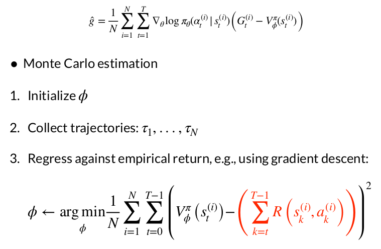
Monte Carlo Value Estimation:

Monte Carlo methods estimate the value of a state by waiting until the episode finishes, then using the actual observed return as the training target.

Intuition: “Don’t guess the future. Wait and see what really happens.”

For a state visited at time $t$, the Monte Carlo return is:

\[G_t=r_t + \gamma r_{t+1} + \gamma^2 r_{t+2} + \dots + \gamma^{T-t} r_T\]

This return is treated as a sample of the true value:

\[V^\pi(s_t) \approx G_t\]

If the value function is parameterized by $\phi$, it can be trained via regression:

\[\mathcal{L}_{MC}(\phi)=\left( V_\phi(s_t) - G_t \right)^2\]

Monte Carlo estimation is:

Unbiased, because it uses the true outcome
High variance, because returns depend on everything that happens later
Delayed, because updates occur only after the episode ends

This makes MC estimation conceptually clean but often impractical for long-horizon or sparse-reward problems.

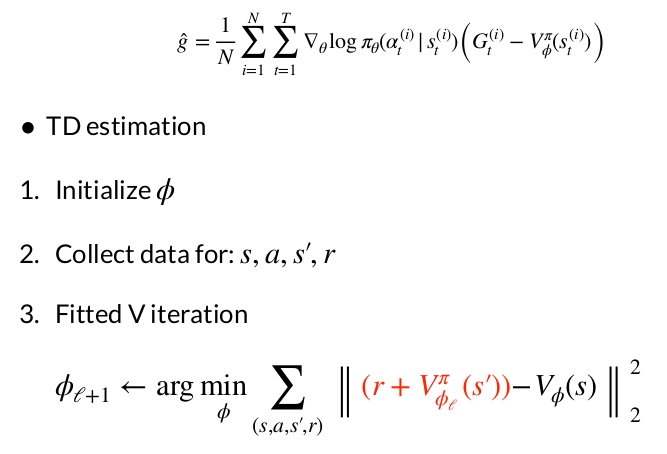
Temporal-Difference (TD) Value Estimation:

Temporal-Difference methods update the value function before the episode ends by bootstrapping from the current value estimate of the next state.

Intuition: “Use what I already believe about the future, and correct myself if I’m wrong.”

Instead of waiting for the full return, TD uses a one-step lookahead:

\[r_t + \gamma V_\phi(s_{t+1})\]

The TD error is defined as:

\[\delta_t=r_t + \gamma V_\phi(s_{t+1}) - V_\phi(s_t)\]

This error measures how surprised the value function is by new experience. The value function is trained to minimize this prediction error:

\[\mathcal{L}_{TD}(\phi)=\delta_t^2\]

Temporal-Difference estimation is:

Lower variance, because it uses shorter-horizon targets
Biased, because it relies on imperfect value estimates
Online, allowing updates at every timestep

In practice, the reduced variance and faster learning usually outweigh the bias.

Once a value function is available, it can be used as a baseline to compute advantages.

Monte Carlo Advantage:

\[A_t^{MC}=G_t - V_\phi(s_t)\]

TD Advantage:

\[A_t^{TD}=r_t + \gamma V_\phi(s_{t+1}) - V_\phi(s_t)\]

A positive advantage $A^{\pi}(s,a) > 0$ means that action $a$ in state $s$ leads to returns higher than the expected value of that state — it’s better than what the policy typically does from that state. A negative advantage means it’s worse. So computing advantages is essentially identifying which actions should be made more likely (positive advantage) and which should be made less likely (negative advantage).

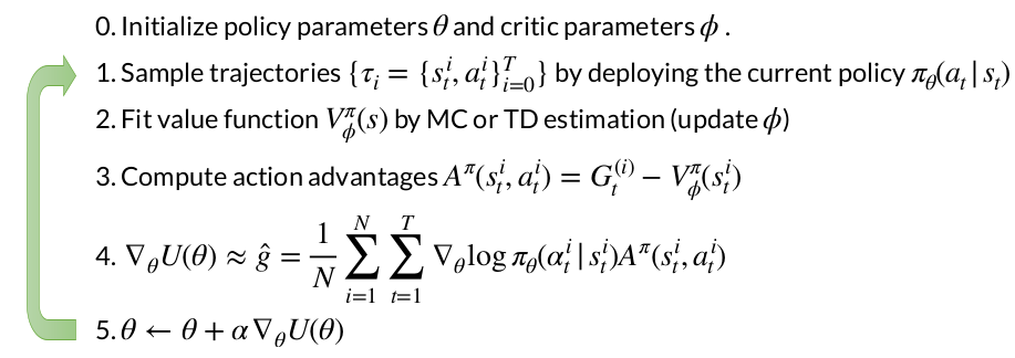
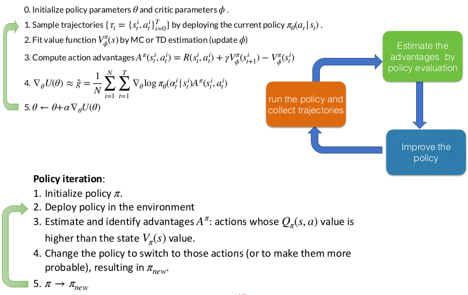
The Core Actor-Critic Framework

Actor-Critic methods maintain two separate components working in tandem: an actor (the policy network) that decides which actions to take, and a critic (the value function network) that evaluates how good those actions are. Think of it like a performer and a coach: the actor performs actions in the environment, while the critic watches and provides feedback on performance. The actor uses this feedback to improve its policy parameters through gradient ascent, while the critic learns to better evaluate states by observing the actual rewards received. In the basic Actor-Critic algorithm, after collecting trajectories by running the current policy, you update the critic to fit a value function $V_{\phi}^{\pi}(s)$ using either Monte Carlo or Temporal Difference estimation. Then, for the policy gradient update, you compute:

\[\nabla_\theta U(\theta) \approx \hat{g} = \frac{1}{N} \sum_{i=1}^{N} \sum_{t=1}^{T} \nabla_\theta \log \pi_\theta(a_t^{(i)} \mid s_t^{(i)}) A^\pi(s_t^{i}, a_t^{i})\]

where the advantage $A^\pi(s_t^i, a_t^i) = G_t^{(i)} - V_{\phi}^{\pi}(s_t^i)$ and $G_t^{(i)}$ is the sample return (the sum of all rewards from time $t$ onward in that trajectory).

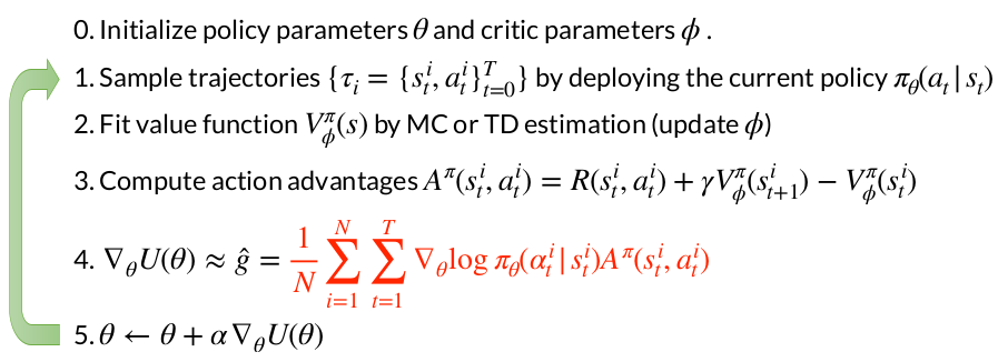
Advantage Actor-Critic (A2C)

The key innovation in A2C is in how it computes the advantage. Instead of using the full Monte Carlo return $G_t$ and subtracting the value function baseline, it uses a bootstrapped estimate. The advantage becomes:

\[A^\pi(s_t^i, a_t^i) = R(s_t^i, a_t^i) + \gamma V_{\phi}^{\pi}(s_{t+1}^i) - V_{\phi}^{\pi}(s_t^i)\]

This is essentially a one-step TD error.

Instead of waiting to collect the entire trajectory’s return, you’re using the immediate reward $R(s_t, a_t)$ plus the estimated value of the next state $\gamma V(s_{t+1})$ and comparing that to your current state’s value $V(s_t)$.

In general, it is useful to remember the following about advantage function:

\[A^\pi(s,a) = Q^\pi(s,a) - V^\pi(s)\] \[\mathbb{E}_{a \sim \pi}[A^\pi(s,a)] = 0\]

Why This Difference Matters: A2C vs AC

The distinction might seem subtle, but it has profound implications for learning efficiency and variance. To understand why, imagine you’re learning to play a game where each episode lasts 1000 steps. In basic Actor-Critic using full returns, the advantage at time step t=5 depends on everything that happens for the next 995 steps. This creates enormous variance. Maybe you made a great move at step 5, but 800 steps later something random happened that ruined the episode. Your advantage estimate would unfairly penalize that early good decision. Advantage Actor-Critic solves this by using the TD error, which essentially asks: “Given what I expected the value of my current state to be, did taking this action and moving to the next state exceed or fall short of expectations?” This is a much more localized signal. You’re only looking one step ahead (or k steps if using k-step returns), and you’re bootstrapping the rest using your learned value function. This dramatically reduces variance at the cost of introducing some bias (since your value function estimate might be wrong). Think of it like getting feedback on your work. Monte Carlo returns (used in basic Actor-Critic) are like waiting until a project is completely finished before getting any evaluation — you get an unbiased assessment, but it’s very noisy because many things could have gone wrong along the way. The TD approach (used in Advantage Actor-Critic) is like getting incremental feedback after each task: “You did better/worse than I expected given where you started.” It’s slightly biased by your coach’s potentially imperfect expectations, but it’s much more consistent and immediate.

From an implementation standpoint, both methods follow similar algorithmic structure — they both initialize policy and critic parameters, sample trajectories, fit the value function, compute advantages, and update the policy. The crucial line that differs is step 3, where advantages are computed.

Actor-Critic as Policy Iteration

Policy iteration alternates between two phases in a loop: policy evaluation and policy improvement. During policy evaluation, you fix your current policy $\pi$ and compute its value function, essentially answering “how good is each state under my current policy?” Then, during policy improvement, you create a new policy that’s greedy with respect to these values, meaning you switch to actions that have higher Q-values than the average. This two-step dance is guaranteed to converge to the optimal policy under certain conditions.

Actor-critic methods implement the same fundamental structure as classical policy iteration, but in a continuous, gradient-based way rather than through discrete policy updates.

The gradient update $\theta \leftarrow \theta + \alpha \nabla_\theta U(\theta)$ increases the probability of actions with positive advantages and decreases the probability of actions with negative advantages. This single update step is the policy improvement. You don’t need to do anything separately. It’s a soft, gradual version of the greedy policy switch in classical policy iteration.

Actor-critic is an on-policy method: you’re evaluating your current policy $\pi_\theta$, computing how good actions are under that specific policy, and then improving that same policy. The data you collected is intrinsically tied to the policy that generated it, just like in policy iteration where $V^{\pi}$ and $Q^{\pi}$ are defined relative to a specific policy $\pi$.

Asynchronous Deep RL for On-Policy Learning

The Core Problem

When training neural networks for reinforcement learning, gradient updates need to be decorrelated for stable learning. However, this creates a fundamental problem for on-policy methods like REINFORCE and actor-critic. When you collect experience sequentially by running a single agent through an environment, consecutive states and actions are highly correlated — each state naturally follows from the previous one. If you compute gradient updates from these sequential, correlated experiences, your value function approximator tends to oscillate and become unstable.

The Asynchronous Solution: Parallel Experience Collection

The key insight of asynchronous deep RL is to parallelize the collection of experience to break these correlations and stabilize training. Instead of running a single agent, you run multiple independent threads of experience simultaneously — one agent per thread. Each agent explores a different part of the environment at the same time, contributing experience tuples (state, action, reward, next state) from diverse regions of the state space. Because these parallel agents are in different states and taking different actions, their experiences are much less correlated than sequential data from a single agent would be.

This approach is particularly crucial for on-policy algorithms like actor-critic because they can’t simply use a replay buffer of old experiences (that would violate the on-policy constraint where data must come from the current policy). Instead, asynchronous parallel collection provides the decorrelation benefits you’d get from experience replay, while still maintaining the on-policy property — all workers are running approximately the same current policy. The diversity comes from spatial exploration across parallel environments rather than temporal diversity from replaying old experiences. The result is much more stable and efficient training. Neural networks converge faster, value function estimates are more accurate, and policies learn more robustly without the wild oscillations that plague sequential single-agent on-policy learning.

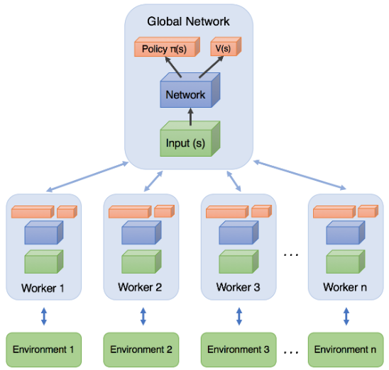
How It Works in Practice

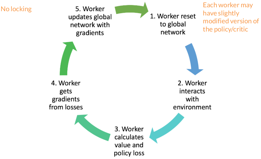
The algorithm runs multiple worker agents in parallel, each with their own copy of the environment. These workers collect trajectories independently and asynchronously. Each worker periodically computes gradients based on its local experience and sends these gradients to a central parameter server (or directly updates shared parameters with appropriate synchronization). The key architectural choice is whether to do this fully asynchronously (A3C - Asynchronous Advantage Actor-Critic) where workers update independently whenever they’re ready, or synchronously (A2C) where all workers wait for each other and their gradients are averaged before updating the central network.

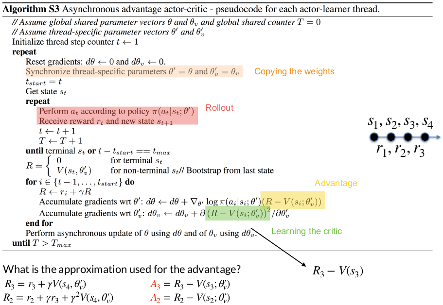
Asynchronous Advantage Actor-Critic (A3C)

Evolutionary Methods for Policy Search

Black-Box Policy Optimization

Black-box policy optimization represents a fundamentally different approach to reinforcement learning compared to the gradient-based methods you’ve studied. Instead of exploiting the structure of the problem (how states connect to each other, how rewards decompose over timesteps), black-box methods treat the entire RL problem as an opaque function to be optimized.

You’re solving:

\[\max_{\theta} U(\theta) = \mathbb{E}_{\tau \sim \pi_\theta} [R(\tau) \mid \pi_\theta, \mu_0(s_0)]\]

You only interact with this objective function by querying it. You try some parameters $\theta$, run the policy, get back a scalar reward $R(\tau)$, and that’s all you know. You don’t compute gradients, you don’t learn value functions, you don’t exploit the Markov structure of the MDP.

Algorithm:

Initialize policy parameters randomly
Perturb the parameters (create variations, mutations, offspring)
Evaluate each perturbed policy by running it in the environment
Select which perturbations led to better performance
Update your parameters toward the better-performing variations
Repeat

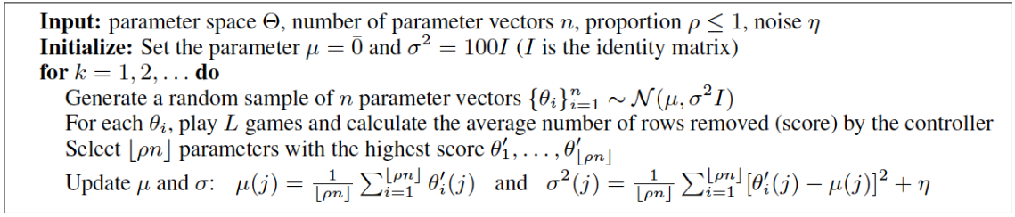
Cross-Entropy Method (CEM)

Principle: keep trying random variations of your policy, remember which ones worked best, and adjust your search distribution to generate more samples like the good ones.

CEM models your policy parameters as random variables drawn from a probability distribution. Specifically, it uses a multivariate Gaussian with a diagonal covariance matrix:

\[\theta \sim \mathcal{N}(\mu, \sigma^2 I)\]

Algorithm:

Initialization: Start with $μ = 0$ and $σ² = 100I$. This means you’re initially searching with a lot of noise, exploring broadly.
Sampling: Generate n random parameter vectors by sampling from your current Gaussian. Think of this as creating $n$ “offspring” or “mutants” of your current best guess:
\[{\theta_i}_{i=1}^n \sim \mathcal{N}(\mu, \sigma^2 I)\]
Evaluation: For each $\theta_i$, run the policy in the environment for $L$ episodes and compute the average score. This is the fitness: how well did that particular parameter vector perform?
Selection: You don’t use all $n$ samples. Instead, you select only the top $[\rho n]$ performers (where $ρ ≤ 1$, typically around 0.1 or 0.2). These are your winners, the parameter vectors that led to the best performance.
Update: Now you shift your search distribution toward these elites. The new mean becomes the average of the elite samples:
\[\mu(j) = \frac{1}{[\rho n]} \sum_{i=1}^{[\rho n]} \theta'_i(j)\]
And the new variance is computed from how spread out the elites are:
\[ \sigma^2(j) = \frac{1}{[\rho n]} \sum_{i=1}^{[\rho n]} [\theta'_i(j) - \mu(j)]^2 + \eta\]
$\eta$ is the added noise to prevent the variance from collapsing to zero, which would kill exploration.

CEM struggles as dimensionality grows. With neural networks having thousands or millions of parameters, the diagonal Gaussian assumption becomes too restrictive, and the selection mechanism (only keeping top $\rho$ fraction) throws away most of your sampled information.

Covariance Matrix Adaptation Evolution Strategy (CMA-ES)

While CEM used a diagonal covariance matrix (assuming parameter independence), CMA-ES uses a full covariance matrix. This means it learns and exploits correlations between parameters, making it dramatically more powerful, though also more complex.

CEM sampled from:

\[ \theta \sim \mathcal{N}(\mu, \sigma^2 I)\]

CMA-ES generalizes this to:

\[\theta \sim \mathcal{N}(\mu, \Sigma)\]

Visual Intuition:

With diagonal covariance (CEM), your search distribution is always axis-aligned — you can only scale search along the coordinate axes. But the optimal search direction might be diagonal.

CMA-ES adapts the ellipse to match the problem geometry. If the fitness landscape is like a valley running northeast-southwest, CMA-ES will stretch its sampling ellipse along that valley. This dramatically improves efficiency because you’re searching along the natural contours of the problem rather than fighting against them.

Algorithm:

Sample: Draw $n$ parameter vectors from your current Gaussian $\mathcal{N}(\mu_i, C_i)$, where $C$ is the covariance matrix at iteration $i$.
Select Elites: Evaluate each sample’s fitness and keep the top performers, just like CEM.
Update Mean: Move your center $\mu$ toward the weighted average of the elite samples:
\[\mu_{t+1} = \mu_t + \alpha \sum_{i=1}^{n_{elit}} w_i(\theta_i^{elit,t} - \mu_t)\]
Update Covariance:
\[ \Sigma_{t+1} = \text{Cov}(\theta_1^{elit,t}, \theta_2^{elit,t}, \ldots) + \epsilon I\]
This tells you: “What directions in parameter space led to good performance?” The covariance matrix encodes these productive search directions. The $\epsilon I$ term (small noise on the diagonal) prevents the matrix from becoming singular.

Natural Evolutionary Strategies (NES)

CEM and CMA-ES had a clear selection mechanism: evaluate samples, keep the elites, throw away the rest. NES takes a different approach: every offspring contributes to the update, weighted by its fitness.

NES maintains a Gaussian distribution over policy parameters, but for computational tractability with neural networks, it uses a diagonal covariance with fixed variance:

\[\theta \sim P_\mu(\theta) = \mathcal{N}(\mu, \sigma^2 I_d)\]

Where:

$\mu \in ℝ^d$ is the mean (what we’re optimizing)
$σ²I_d$ is a fixed diagonal covariance ($\sigma$ is a hyperparameter)
$d$ is the parameter dimension

The goal is to maximize the expected fitness:

\[\max_\mu U(\mu) = \mathbb{E}_{\theta \sim P\mu(\theta)} [F(\theta)]\]

where $F(\theta)$ is the fitness (total return) when running policy $\pi \theta$.

Derivation

\[\nabla_\mu U(\mu) = \nabla_\mu \mathbb{E}_{\theta \sim P\mu(\theta)} [F(\theta)]\]

We can write the expectation as an integral:

\[\nabla_\mu U(\mu) = \nabla_\mu \int P_\mu(\theta) F(\theta) d\theta\] \[= \int \nabla_\mu P_\mu(\theta) F(\theta) d\theta\]

Log-likelihood trick:

\[\nabla_\mu U(\mu) = \int P_\mu(\theta) \frac{\nabla_\mu P_\mu(\theta)}{P_\mu(\theta)} F(\theta) d\theta\] \[= \int P_\mu(\theta) \nabla_\mu \log P_\mu(\theta) F(\theta) d\theta\] \[= \mathbb{E}_{\theta \sim P\mu(\theta)} [\nabla_\mu \log P_\mu(\theta) F(\theta)]\]

This is exactly the same trick used in policy gradients! Just like REINFORCE transforms policy gradients into an expectation, NES transforms parameter distribution gradients into an expectation.

Since we have an expectation, we can approximate it by sampling:

\[ \nabla_\mu U(\mu) \approx \frac{1}{N} \sum_{i=1}^N \nabla_\mu \log P_\mu(\theta^{(i)}) F(\theta^{(i)})\]

where each $\theta^i \sim P_\mu(\theta)$.

For our Gaussian with mean $\mu$ and fixed variance $\sigma^2I$:

\[ \log P_\mu(\theta) = -\frac{|\theta - \mu|^2}{2\sigma^2} + \text{const}\]

Taking the gradient with respect to $\mu$:

\[\nabla_\mu \log P_\mu(\theta) = \frac{\theta - \mu}{\sigma^2}\]

So the NES update becomes:

\[\mu_{t+1} = \mu_t + \frac{\alpha}{N\sigma} \sum_{i=1}^N F(\theta_i) \epsilon_i\]

where $\theta_i = \mu_t + \sigma \epsilon_i$ and $\epsilon_i \sim \mathcal{N}(0,I)$.

Value-Based RL

Review: Actor-Critic and the Advantage Function

We saw previously that in actor-critic methods, we’re optimizing a policy gradient objective that looks like this:

\[\nabla_\theta U(\theta) = \mathbb{E}_{\tau \sim \pi_\theta(\tau)} \left[ \sum_{t=0}^{T} \nabla_\theta \log \pi_\theta(a_t \mid s_t) \cdot A^{\pi}(s_t, a_t) \right]\]

The advantage function plays a crucial role here, serving as our signal for which actions are better than average. The advantage is formally defined as:

\[A^{\pi}(s_t, a_t) = r(s_t, a_t) + \gamma V^{\pi}(s_{t+1}) - V^{\pi}(s_t)\]

Intuition: The term $r(s_t, a_t) + \gamma V^\pi(s_{t+1})$ represents the Q-value of the state-action pair, essentially asking “what’s the total expected return if I take action $a_t$ in state $s_t$ and then follow $\pi$ afterward?” By subtracting the value function $V^\pi(s_t)$, which represents the average value of being in that state, we get a relative measure. The advantage tells us: “how much better is this specific action compared to what we’d typically expect in this state?”

We can also express the advantage function in terms of Q-values and values:

\[A^{\pi}(s_t, a_t) = Q^{\pi}(s_t, a_t) - V^{\pi}(s_t)\]

General policy-based RL workflow:

We collect trajectories by rolling out our current policy in the environment
We estimate how good each action was by computing returns or advantages through policy evaluation
We improve the policy by adjusting it to favor actions with higher estimated advantages.

The Value-Based Approach

Now we arrive at a fundamental question that motivates value-based RL: if we had a perfect estimate of the advantage function, would we even need to maintain an explicit policy? The answer is no, and this insight drives the entire value-based methodology.

Think about it this way: in policy-based methods, we’re using the advantage estimates to nudge our policy parameters gradually in the direction of better actions. We collect data, estimate advantages using rollouts from our policy, compute gradients, and take small steps. But if we somehow had perfect knowledge of $A^\pi(s,a)$ for all state-action pairs, we could simply construct the optimal policy by taking the argmax:

\[\pi(s) \leftarrow \argmax_a A^\pi(s,a)\]

This leads to the value-based RL skeleton, which differs from policy-based methods primarily in steps 2 and 3:

Collect data in the environment using the current policy $\pi$ (with some exploration noise to ensure we visit diverse states).
Estimate the advantage function $A^\pi(s,a)$ as perfectly as possible rather than just well enough to compute a policy gradient. This is where we invest most of our effort by building the most accurate model we can of which actions are truly better.
Update the policy via argmax by setting $\pi’(s) = \argmax_a A^\pi(s, a)$ for all states. Notice this is “off-policy” in the sense that we’re not computing gradients of the policy itself; we’re simply choosing the best action according to our learned advantage estimates.

We don’t need to worry about policy parameterization, gradient estimation, or learning rates for the policy. If our advantage estimates are good, the policy update is trivial — just pick the best action.

Value Iteration and Q-Learning

The theoretical algorithm that formalizes this idea is called dynamic programming or value iteration. The core of value iteration is the Bellman equation for the Q-function:

\[Q(s, a) = r(s, a) + \gamma \mathbb{E}_{s' \sim p(\cdot \mid s, a)} [V(s')]\]

Intuition: “The value of taking action $a$ in state $s$ equals the immediate reward plus the discounted expected value of wherever we end up next.”

The value iteration algorithm alternates between two updates:

Update 1: Update Q-values using the Bellman equation:
\[Q(s, a) \leftarrow r(s, a) + \gamma \mathbb{E}_{s'} [V(s')]\]
Update 2: Update the value function by taking the max over actions:
\[V(s) \leftarrow \max_a Q(s, a)\]

These updates are performed iteratively until convergence. In tabular settings (where we have finite state and action spaces), we can literally maintain a table with entries $Q(s, a)$ for every possible state-action pair, and this algorithm is guaranteed to converge to the optimal Q-function.

But here’s the practical challenge: how do we implement this when we have large or continuous state spaces? We need function approximation.

Fitted Q-Iteration: Neural Networks for Value Functions

To scale value-based methods to complex domains, we use neural networks to approximate the Q-function. This leads to fitted Q-iteration, where instead of maintaining a table, we train a neural network $Q_\theta(s,a)$ parameterized by weights $\theta$.

The training procedure draws inspiration from supervised learning, specifically, from temporal difference (TD) learning. Here’s how it works:

We want to train $Q_\theta$ to satisfy the Bellman equation, so we construct a target value:

\[y(s, a) = r(s, a) + \gamma \max_{a'} Q_\theta(s', a')\]

The target itself involves our Q-function evaluated at the next state $s’$. This creates a “bootstrap” situation where we’re using our current estimates to create training targets for future estimates.

We then define a TD-error loss function which we want to minimize:

\[\text{TD-Error}(\theta) = \mathbb{E}_{s, a, s' \sim \mathcal{D}} \left[ \left( Q_\theta(s, a) - y(s, a) \right)^2 \right]\]

The gradient update becomes:

\[\theta_{t+1} \leftarrow \theta_t - \alpha \nabla_\theta \text{TD-Error}(\theta) \big|_{\theta = \theta_t}\]

This is not gradient descent in the traditional sense. Why? Because our target $y(s,a)$ itself depends on $\theta$ through the $\max_{a’} Q_\theta(s’, a’)$ term. When we compute the gradient, we’re treating the target as fixed (not differentiating through it), but the target is actually moving as $\theta$ changes. This creates a moving target problem that can lead to instability.

Think of it like trying to hit a bullseye that keeps shifting position as you aim. Traditional supervised learning has a fixed target. But in Q-learning, as our Q-estimates get better, the targets we’re aiming for also change, creating a feedback loop that can sometimes diverge.

Despite this theoretical concern, fitted Q-iteration can work in practice with the right tricks. The key insight is that even though we’re not doing true gradient descent on a fixed objective, we’re still iteratively improving our Q-estimates to better satisfy the Bellman equation.

Why the Q-Learning Target Makes Sense:

The target $y(s, a) = r(s, a) + \gamma \max_{a’} Q(s’, a’)$ comes directly from the Bellman optimality equation. When you take action $a$ in state $s$, your total expected return naturally splits into two components: the immediate reward $r(s,a)$ you receive right now, and the best possible future value you can obtain from wherever you land next, which is $\gamma \max_{a’} Q(s’, a’)$. The max operator appears because we’re learning the optimal Q-function, which assumes we’ll always choose the best action going forward, even if our current exploratory policy doesn’t actually do that yet.

This creates a bootstrapping process where we use our current value estimates to improve themselves. Even though our Q-estimates start out imperfect, we can make progress by using the estimate at the next state $s’$ to improve the estimate at the current state $s$. The one-step reward $r(s,a)$ provides accurate immediate information, and combining it with our (gradually improving) estimate of future value pushes our Q-function toward satisfying the Bellman equation. Over many iterations, these improvements propagate backward through the state space, eventually converging to the optimal Q-function.

The reason we take the max rather than averaging over our current policy’s action distribution is what makes Q-learning “off-policy” — it learns about the optimal policy directly, regardless of how we’re actually behaving during data collection. This allows us to learn from exploratory or even random actions, since we’re always targeting what the best action would be, not what we actually did.

Deep Q-Networks (DQN)

The breakthrough that made deep Q-learning practical came with the Deep Q-Network (DQN) algorithm, which introduced two critical innovations to address the instability issues.

Innovation 1: Replay Buffer

Instead of training on data as it comes from the agent’s current policy, DQN stores transitions (s, a, r, s') in a large replay buffer (essentially a dataset of experiences). During training, we sample random mini-batches from this buffer rather than using consecutive experiences.

Why does this help?

First, it breaks the correlation between consecutive samples. If we trained on experiences in the order they occurred, the network would see highly correlated data (e.g., many frames from the same episode of a game), which can lead to overfitting to recent experiences and catastrophic forgetting of earlier lessons. Random sampling from the replay buffer gives us more independent and identically distributed-like data, which neural networks handle much better.

Second, the replay buffer provides data efficiency. Each experience can be used for multiple gradient updates rather than being discarded after a single use. This is particularly valuable in domains where collecting data is expensive.

Innovation 2: Target Networks

To address the moving target problem, DQN maintains two sets of Q-network parameters: the current network $\theta_t$ that we’re actively training, and a target network $\theta_t^{target}$ that we use to compute the targets in the Bellman equation.

The TD-error loss now becomes:

\[\min_\theta \mathbb{E}_{(s, a, r, s') \in \mathcal{D}} \left[ \left( Q_\theta(s, a) - \left( r(s, a) + \gamma \max_{a'} Q_{\theta_t^{\text{target}}}(s', a') \right) \right)^2 \right]\]

The key idea is that we update $\theta_t$ on every gradient step, but we only update the target network $\theta_t^{target}$ occasionally (e.g., every few thousand steps) by copying the current network weights. This creates a period of stability where the targets remain fixed while we train, reducing the moving target problem. It’s like the bullseye staying still for a while so we can actually learn to aim at it before it moves again.

Algorithm

The complete DQN algorithm works as follows:

Collect data using policy $\pi_{\theta_t}$ (typically $\epsilon-$greedy: take argmax action with probability $1-\epsilon$, and random action with probability $\epsilon$ for exploration by sampling from a uniform distribution of actions $\pi \sim \text{Unif}(\mathcal{A})$ ).
\[\pi(s) = \arg\max_{a'} Q_{\theta_t}(s, a')\]
Store transitions (s, a, r, s') in replay buffer $\mathcal{D}$
Sample mini-batch from $\mathcal{D}$ and perform gradient descent on:
\[\min_\theta \mathbb{E}_{(s, a, r, s') \in \mathcal{D}} \left[ \left( Q_\theta(s, a) - \left( r(s, a) + \gamma \max_{a'} Q_{\theta_t^{\text{target}}}(s', a') \right) \right)^2 \right]\]
Periodically update target network: every $K$ steps, set $\theta_t^{target} \leftarrow \theta_t$

The use of soft targets (keeping the target network fixed for periods) combined with the replay buffer’s decorrelated sampling creates a much more stable training process than naive fitted Q-iteration. This allowed DQN to achieve superhuman performance on many Atari games, marking a major milestone in deep reinforcement learning.

The fundamental insight of DQN is that even though we’re not doing true gradient descent (since we’re using target networks and treating parts of our objective as fixed), we can still make meaningful progress by carefully managing the optimization process to reduce instability.

Key Hyperparameters and Design Choices

Update-to-Data (UTD) Ratio:

The UTD ratio measures how many gradient updates we perform per environment step. If UTD = 1, we take one gradient step for each new transition we collect. If UTD = 4, we perform four gradient updates (sampling four different mini-batches from the replay buffer) for each new transition.

A higher UTD ratio means we’re extracting more learning from each piece of data, which can be sample-efficient. However, there’s a trade-off: if the UTD ratio is too high, we can overfit to the data in our replay buffer, and the rapid updates can destabilize training. The agent might start exploiting patterns in old data that are no longer relevant to the current policy. Selecting its value is problem-dependent, as there are cases where UTD is as high as 100, but sometimes as low as 0.001.

Example scenario for UTD=4. So the process looks like this:

Agent takes one action in environment $\rarr$ gets one new transition $\rarr$ add it to replay buffer
Sample mini-batch #1 from replay buffer $\rarr$ compute loss $\rarr$ gradient step
Sample mini-batch #2 from replay buffer $\rarr$ compute loss $\rarr$ gradient step
Sample mini-batch #3 from replay buffer $\rarr$ compute loss $\rarr$ gradient step
Sample mini-batch #4 from replay buffer $\rarr$ compute loss $\rarr$ gradient step
Return to step 1, take another action in environment

Those 4 gradient steps in the middle are all training on old data from the replay buffer, not on the single new transition we just collected. The new transition goes into the buffer and might get sampled in future mini-batches, but we’re primarily learning from historical experiences.

Hard vs Soft Target Updates

The target network update described above is called a “hard update”, where we completely replace $\theta^{target}$ with $\theta$ all at once. An alternative approach is “soft updates,” where we gradually blend the target network toward the main network at every step:

\[\theta^{\text{target}}_{i+1} \leftarrow (1 - \alpha) \theta^{\text{target}}_i + \alpha \theta_i\]

Here $\alpha$ is a small constant like 0.005. This means the target network slowly tracks the main network, providing continuously updating targets rather than sudden jumps. Hard updates every $K$ steps with $K$ large create discrete jumps, while soft updates with small $\alpha$ create smooth tracking. Soft updates often provide more stable training because the targets change gradually rather than suddenly shifting every few thousand steps.

Note: You pick one strategy and stick with it throughout training. They’re two different design choices for solving the same problem (keeping targets stable), not complementary techniques you’d combine.

Challenges with DQN

Challenge 1: Overestimation Bias in Q-Values

One of the major practical challenges with DQN is that it tends to systematically overestimate Q-values. This is a fundamental issue with how the algorithm compounds errors through bootstrapping.

The Root Cause: Error Accumulation Through Max Operations

Our target is:

\[y(s,a) = r(s,a) + \gamma \max_{a'} Q_{\theta^{\text{target}}}(s', a')\]

The term $\max_{a’} Q_{\theta^{target}}(s’, a’)$ is supposed to represent the optimal state value $V^*(s’)$, which is the true value we’d get by following the optimal policy from state $s’$ onward. However, our Q-function $Q_{\theta^{target}}$ is not perfect and has some errors. Some actions might have Q-values that are too high (overestimates), while others might be too low (underestimates).

This problem becomes serious because we’re doing bootstrapping — the Q-value we’re training becomes the target for earlier states. So if $Q_\theta(s’, a’)$ is overestimated, then when we compute the target for state $s$, we use this overestimate. This means $Q_\theta(s, a)$ will also become overestimated. Then when we compute targets for states that lead to $s$, they inherit this error, and so on. The overestimation compounds backward through the state space like a chain reaction.

Double DQN: Decoupling Action Selection and Evaluation

The problem is that we’re using the same Q-function both to select which action looks best AND to evaluate how good that action is. This creates the bias—we pick the action with the largest estimation error, then trust that error as our target.

Double DQN fixes this by maintaining two Q-functions (initialized differently): $Q_{\theta^A}$ and $Q_{\theta^B}$. The key idea is to use one network to select the action and the other network to evaluate it. Here’s how the target computation changes:

Use network A to determine which action looks best in state $s’$:
\[a^* = \arg\max_{a} Q_{\theta^A}(s', a)\]
Use network B to evaluate that specific action:
\[y(s,a) = r(s,a) + \gamma Q_{\theta^B}(s', a^*)\]

Why does this help? If network A has a positive error on some action (thinks it’s better than it really is), it will select that action. But then network B evaluates it, and B’s errors are independent of A’s errors (since they were initialized differently and trained on different mini-batches). So B is unlikely to have the same overestimation for that same action. On average, this decorrelates the selection bias from the evaluation bias, dramatically reducing the systematic overestimation.

In practice with DQN, we already have two networks—the main network $\theta$ and the target network $\theta^{target}$ — so we can implement Double DQN without adding any extra parameters. We use the main network to select actions and the target network to evaluate them:

\[a^* = \arg\max_{a} Q_{\theta}(s', a)\] \[y(s,a) = r(s,a) + \gamma Q_{\theta^{\text{target}}}(s', a^*)\]

Challenge 2: Reducing Error Compounding with N-Step Returns

Another approach to reducing error accumulation is to use N-step returns instead of one-step TD targets. The standard DQN target uses only one step of real reward before bootstrapping:

\[y(s,a) = r(s,a) + \gamma \max_{a'} Q_{\theta^{\text{target}}}(s', a')\]

This means we trust the immediate reward $r(s,a)$ (which comes from the environment and is accurate), but then immediately rely on our Q-function estimate for everything after. If our Q-estimates are poor, this propagates error quickly.

With N-step returns, we instead accumulate N steps of actual rewards before bootstrapping. If we have a trajectory (s, a, r, s', a', r', s'', ...) in our replay buffer, we can construct an N-step target:

\[y_N(s,a) = r(s,a) + \gamma r(s', a') + \gamma^2 r(s'', a'') + \cdots + \gamma^N \max_{a} Q_{\theta^{\text{target}}}(s_{N+1}, a)\]

The intuition is that we’re trusting real data for longer before falling back on our potentially erroneous estimates.

The trade-off is that N-step returns introduce higher variance — they depend on N different random rewards and state transitions — and they can only be computed for transitions where we have N subsequent steps stored in the replay buffer. But when tuned properly, they often significantly improve learning by reducing the impact of Q-value errors on the targets. The most common value of N used in practice is 3.

Challenge 3: Cold Start Problem

At the very beginning of training, the replay buffer is empty, so DQN cannot perform any updates. The solution is a burn-in phase: before any Q-network training begins, the agent collects an initial dataset by acting in the environment for thousands of steps using either a random policy or highly exploratory $\epsilon-$greedy policy. This fills the replay buffer with diverse experiences. Only after this warm-up period do gradient updates begin. The Q-network starts with random weights and poor predictions, but it now has real environmental data to learn from.

Challenge 4: The Limited Exploration Problem

A more persistent challenge arises when the agent repeatedly visits similar states and fails to explore broadly. This can happen if the policy is too exploitative ($\epsilon$ too small), if certain states act as “attractors” where the agent gets stuck, or if the state space is so vast that the explored region remains limited. When the replay buffer lacks diversity, the Q-function becomes specialized to only the visited states and performs poorly elsewhere, trapping the agent in a local optimum where its policy keeps leading it back to the same familiar territory.

This is why $\epsilon-$greedy exploration is essential throughout training. With probability $\epsilon$, the agent takes random actions instead of greedy ones, occasionally forcing it out of comfortable patterns and into new situations. In practice, $\epsilon$ typically starts at 1.0 during burn-in, then gradually decays to a small constant like 0.1 or 0.05. This schedule prioritizes early exploration to build buffer diversity, then shifts toward exploitation as the Q-function improves, while maintaining baseline exploration indefinitely to prevent getting stuck. Even a small constant $\epsilon$, over millions of steps, generates enough random detours to gradually expand the explored region and diversify the replay buffer.

Practical Training Details for DQN

A few additional implementation details that significantly impact DQN’s performance:

Coverage Really Helps: Ensuring broad state-space coverage through effective exploration is crucial. If the replay buffer only contains data from a limited region of the state space, the Q-function will have poor estimates elsewhere, and the agent may fail to discover better behaviors. Techniques like decaying $\epsilon$ over time (starting with high exploration, gradually reducing it as we learn) help balance initial exploration with later exploitation.

High UTD Can Destabilize Training: While performing many gradient updates per environment step seems attractive for sample efficiency, setting the UTD ratio too high can cause instability. The agent essentially overfits to its replay buffer, and rapid Q-value changes can violate the assumptions that make target networks helpful. Conservative UTD ratios tend to be more robust.

Improved Loss Functions: Instead of using standard squared error, practitioners often use the Huber loss, which is quadratic for small errors but linear for large errors:

\[L(x) = \begin{cases}\frac{x^2}{2}, & |x| \leq \delta \\\delta |x| - \frac{\delta^2}{2}, & |x| > \delta\end{cases}\]

In the context of DQN, $x$ represents the TD-error:

\[x = Q_{\theta}(s,a) - \left( r + \gamma \max_{a'} Q_{\theta^{\text{target}}}(s', a') \right)\]

$\delta(x)$ is a hyperparameter that we choose.

This makes training more robust to outliers and large TD-errors, which can occur especially early in training when Q-estimates are poor. The Huber loss prevents single large errors from causing dramatic parameter updates that destabilize learning.

Understanding $V(s)$ in Value-Based RL

$V(s)$ is Implicitly Computed, Not Separately Stored

In DQN, we only learn the Q-function $Q_\theta(s,a)$ using a neural network. We don’t maintain a separate value function. However, $V(s)$ isn’t missing. It is simply computed implicitly whenever we need it through the relationship:

\[V(s) = \max_a Q_\theta(s, a)\]

This means $V(s)$ automatically stays synchronized with our Q-values. Every time the parameters $\theta$change and our Q-function improves, the value function $V(s)$ implicitly changes along with it because it’s derived from the Q-values. We’re not storing two separate functions that could fall out of sync; we’re storing one function (Q) and computing the other (V) from it on-demand (if at all needed).

Why Advantages and Q-Values Lead to the Same Policy

The advantage function is defined as $A(s,a) = Q(s,a) - V(s)$. You might wonder whether we should be taking the argmax over advantages or over Q-values. The answer is that it doesn’t matter, since they give the same result.

When we’re selecting an action, we compute $\argmax_a A(s,a) = \argmax_a [Q(s,a) - V(s)]$. The critical observation is that $V(s)$ is the same value for all actions in state $s$ at any given moment in time. Since $V(s)$ doesn’t depend on which action we’re considering, it’s just a constant that gets subtracted from all Q-values equally. Adding or subtracting the same constant from every option doesn’t change which option is largest, so:

\[\argmax_a [Q(s,a) - V(s)] = \argmax_a Q(s,a)\]

This is why DQN can work directly with Q-values for action selection without ever explicitly computing advantages. The policy is simply:

\[\pi(s) = \argmax_a Q_\theta(s,a)\]

Advanced Policy Gradients: Bridging Policy-Based and Value-Based Methods

Motivation

Up to this point, we’ve studied two distinct families of reinforcement learning algorithms. Policy gradient methods learn an explicit policy (perhaps with an on-policy value function for variance reduction), and they’re fundamentally on-policy — they must collect data using the current policy being optimized. Value-based methods like Q-learning don’t maintain an explicit policy at all; instead, they learn a value function and derive the policy implicitly through argmax operations, which allows them to be off-policy and leverage replay buffers for sample efficiency.

A natural question arises: can we build a hybrid that combines the best of both worlds? Such an algorithm should be off-policy to benefit from replay buffers and reuse old data, yet it should maintain an explicit policy network that we can optimize using actor-critic style updates. This would give us the expressiveness and continuous action handling of policy gradients with the sample efficiency of value-based methods. The answer is yes, and this leads us to a family of algorithms called off-policy policy gradient methods. The challenge is: how do we derive a principled way to make this work?

The Performance Difference Lemma

The key mathematical tool that enables off-policy policy gradients is the Performance Difference Lemma. This lemma provides an exact relationship between the performance of any two policies $\pi$ and $\mu$.

Recall that the advantage function for a policy $\mu$ is defined as:

This measures how much better action $a$ is compared to the average value of being in state $s$ under policy $\mu$. Importantly, we have the property that the expected advantage under the policy’s own action distribution is zero:

This is because when we average the advantage over all actions weighted by how often the policy takes them, the positive and negative deviations from the mean cancel out.

Now, the Performance Difference Lemma states that for any two policies $\pi$ (the policy we’re evaluating) and $\mu$ (some other policy), the difference in their expected returns can be expressed as:

What the above equation means: The trajectories $\tau$ are generated by following policy $\pi$ (so states are distributed according to $\pi$’s state visitation), but the advantages being summed are computed with respect to policy $\mu$. It connects the performance of $\pi$ to advantages measured under a different policy $\mu$.

Why is this useful? This lemma tells us that to improve $\pi$ relative to $\mu$, we want to maximize the expected sum of $\mu$’s advantages along trajectories generated by $\pi$. If we can accurately estimate $A^\mu$ (using a critic), we can optimize $\pi$ to take actions that have high advantage according to $\mu$.

Derivation

We start with the definition of the return:

\[J(\pi) = \mathbb{E}_{\tau \sim p_{\pi}(\tau)} \left[ \sum_{t=0}^{\infty} \gamma^t r(s_t, a_t) \right]\]

Now, notice that the entire sum of rewards is just $V^\pi(s_0)$, the value of the initial state under policy $\pi$. So we can write:

\[J(\pi) = \mathbb{E}_{s_0 \sim p(s_0)} [V^{\pi}(s_0)]\]

The key insight here is that the trajectory distribution $p_\pi(\tau)$ can be decomposed: first we sample $s_0$ from some initial state distribution $p(s_0)$, and then the rest of the trajectory unfolds according to $\pi$. Since $s_0$ is sampled independently of the policy, the expectation over trajectories becomes an expectation over just the initial state.

Similarly, for policy $\mu$:

\[J(\mu) = \mathbb{E}_{s_0 \sim p(s_0)} [V^{\mu}(s_0)]\]

Now let’s compute the difference:

\[J(\pi) - J(\mu) = \mathbb{E}_{s_0 \sim p(s_0)} [V^{\pi}(s_0)] - \mathbb{E}_{s_0 \sim p(s_0)} [V^{\mu}(s_0)]\]

Since both expectations are over the same distribution, we can combine them:

\[J(\pi) - J(\mu) = \mathbb{E}_{s_0 \sim p(s_0)} [V^{\pi}(s_0) - V^{\mu}(s_0)]\]

We want to express this difference in terms of advantages. To do this, we need to “unroll” the value function recursively using the Bellman equation.

Recall the Bellman equation for $V^\pi$:

\[V^{\pi}(s) = \mathbb{E}_{a \sim \pi(\cdot|s), s' \sim p(\cdot|s,a)} [r(s,a) + \gamma V^{\pi}(s')]\]

Let’s apply this to $s_0$:

\[V^{\pi}(s_0) = \mathbb{E}_{a_0 \sim \pi(\cdot|s_0), s_1 \sim p(·|s_0, a_0)} [r(s_0, a_0) + \gamma V^{\pi}(s_1)]\]

Now we want to introduce $V^\mu$ into this expression. Notice that we can write:

\[V^{\pi}(s_0) - V^{\mu}(s_0) = \mathbb{E}_{a_0 \sim \pi, s_1} [r(s_0, a_0) + \gamma V^{\pi}(s_1)] - V^{\mu}(s_0)\] \[V^{\pi}(s_0) - V^{\mu}(s_0) = \mathbb{E}_{a_0 \sim \pi, s_1} [r(s_0, a_0) + \gamma V^{\pi}(s_1) - \gamma V^{\mu}(s_1) + \gamma V^{\mu}(s_1)] - V^{\mu}(s_0)\]

Rearranging:

\[V^{\pi}(s_0) - V^{\mu}(s_0) = \mathbb{E}_{a_0 \sim \pi, s_1} [r(s_0, a_0) + \gamma V^{\mu}(s_1) - V^{\mu}(s_0) + \gamma(V^{\pi}(s_1) - V^{\mu}(s_1))]\]

Recall that:

\[A^{\mu}(s_0, a_0) = Q^{\mu}(s_0, a_0) - V^{\mu}(s_0) = r(s_0, a_0) + \gamma V^{\mu}(s_1) - V^{\mu}(s_0)\] \[V^{\pi}(s_0) - V^{\mu}(s_0) = \mathbb{E}_{a_0 \sim \pi, s_1} [A^{\mu}(s_0, a_0) + \gamma(V^{\pi}(s_1) - V^{\mu}(s_1))]\]

Now we have a recursive structure. The last term $\gamma (V^\pi(s_1) - V^\mu(s_1))$ has the same form as what we started with, just at time step 1 instead of time step 0. We can apply the same trick again:

\[V^{\pi}(s_1) - V^{\mu}(s_1) = \mathbb{E}_{a_1 \sim \pi, s_2} [A^{\mu}(s_1, a_1) + \gamma(V^{\pi}(s_2) - V^{\mu}(s_2))]\]

Substituting this back:

\[V^{\pi}(s_0) - V^{\mu}(s_0) = \mathbb{E}_{a_0 \sim \pi, s_1} [A^{\mu}(s_0, a_0) + \gamma \mathbb{E}_{a_1 \sim \pi, s_2} [A^{\mu}(s_1, a_1) + \gamma(V^{\pi}(s_2) - V^{\mu}(s_2))]]\]

Distributing the outer expectation and the $\gamma$:

\[V^{\pi}(s_0) - V^{\mu}(s_0) = \mathbb{E}_{a_0 \sim \pi, s_1} [A^{\mu}(s_0, a_0)] + \gamma \mathbb{E}_{a_0 \sim \pi, s_1, a_1 \sim \pi, s_2} [A^{\mu}(s_1, a_1)] + \gamma^2 \mathbb{E}_{...} [V^{\pi}(s_2) - V^{\mu}(s_2)]\]

If we keep expanding this pattern infinitely (which is valid as long as $\gamma <1$ ensures convergence), we get:

\[V^{\pi}(s_0) - V^{\mu}(s_0) = \sum_{t=0}^{\infty} \gamma^t \mathbb{E}_{s_0, a_0, s_1, a_1, ..., s_t, a_t} [A^{\mu}(s_t, a_t)]\]

where the expectation is taken over trajectories generated by policy $\pi$ (so $s_0 \sim p(s_0)$, then $a_0 \sim \pi(\cdot

s_0)$, then $s_1 \sim p(\cdot

s_0,a_0)$, and so on).

We can write this more compactly as:

\[V^{\pi}(s_0) - V^{\mu}(s_0) = \mathbb{E}_{\tau \sim p_{\pi}(\tau)} \left[ \sum_{t=0}^{\infty} \gamma^t A^{\mu}(s_t, a_t) \right]\]

Finally, we take the expectation over the initial state distribution:

\[J(\pi) - J(\mu) = \mathbb{E}_{s_0 \sim p(s_0)} [V^{\pi}(s_0) - V^{\mu}(s_0)]\] \[= \mathbb{E}_{s_0 \sim p(s_0)} \left[ \mathbb{E}_{\tau \sim p_{\pi}(\tau)} \left[ \sum_{t=0}^{\infty} \gamma^t A^{\mu}(s_t, a_t) \right] \right]\] \[J(\pi) - J(\mu) = \mathbb{E}_{\tau \sim p_{\pi}(\tau)} \left[ \sum_{t=0}^{\infty} \gamma^t A^{\mu}(s_t, a_t) \right]\]

The Optimization Problem

The Performance Difference Lemma gives us an exact expression for $J(\pi) - J(\mu)$, but how do we use this to actually optimize $\pi$? We can frame this as a constrained optimization problem:

But there’s a catch: the expectation is over trajectories sampled from $\pi$. This means to evaluate this expression, we need to actually run policy $\pi$ in the environment, collect full trajectories, and compute advantages along those trajectories. Every time we update $\pi$, we’d need fresh data from the new $\pi$. This is on-policy learning, and it is sample-inefficient because we can’t reuse old data.

When we write $\tau \sim p_\pi(\tau)$, we’re sampling an entire trajectory according to $\pi$’s distribution. But what does this really mean? A trajectory is a sequence $(s_0, a_0, s_1, a_1, s_2, a_2, …)$, and the distribution over trajectories can be factored:

First, we sample $s_0$ from the initial state distribution $p(s_0)$
Then we sample $a_0$ from $\pi(\cdot s_0)$
Then the environment gives us $s_1$ from $p(\cdot s_0, a_0)$
Then we sample $a_1$ from $\pi(\cdot s_1)$
And so on…

The key is that which states we visit is determined by the policy. Policy $\pi$ creates a specific pattern of state visitation over time. We call this the “state visitation distribution” or “state marginal distribution” and denote it $p_\pi(s_t)$ for time step $t$, or more generally $d^\pi(s)$ for the discounted state visitation.

Here’s where we make a crucial approximation that enables off-policy learning. Instead of collecting data under $\pi$ (the policy we’re optimizing), we can collect data under $\mu$ (some behavioral policy, perhaps an older version of $\pi$) and correct for the distribution mismatch. We rewrite the expectation over $\pi$’s trajectories as:

This approximation says: instead of following $\pi$’s entire trajectory distribution (which determines which states we visit), we use states visited by $\mu$, but we still choose actions according to $\pi$ at each state. The key insight is that when $\pi$ and $\mu$ are close (which we’ll enforce with a constraint), the states visited by the two policies are similar, so this approximation is reasonable.

Now the inner expectation only involves sampling actions from $\pi$ given states from $\mu$’s distribution:

\[\mathbb{E}_{s \sim d^{\mu}(s)} \left[ \mathbb{E}_{a \sim \pi(\cdot|s)} [A^{\mu}(s, a)] \right]\]

where $d^\mu(s)$ represents the discounted state visitation distribution under policy $\mu$. This is something we can estimate from a replay buffer filled with $\mu$’s experiences.

We add a constraint to keep $\pi$ close to $\mu$, typically measured by a divergence $D(\pi,\mu)$. This gives us the constrained optimization problem:

where $\alpha$ controls how much we penalize deviation from $\mu$. The divergence $D$ can be chosen in different ways, such as KL divergence, total variation distance, etc., and each choice leads to a different algorithm.

If $D(\pi(\cdot

s), \mu(\cdot

s))$ is small, then it implies that $p_\pi(s) \sim p_\mu(s)$.

Some Additional Math

The left side sums over time steps in a trajectory. The right side removes the explicit time dependence by using the discounted state visitation distribution $d^\pi(s)$.

The discounted state visitation distribution $d^\pi(s)$ is defined as:

This is a distribution (not just a sum) because of the normalization factor $(1-\gamma)$. It represents “how often do we visit state $s$, weighted by how far in the future it is.” The factor $(1-\gamma)$ ensures that when we sum over all states $s$, we get $1$ (a valid probability distribution).

Let’s start with the left side and manipulate it:

\[\mathbb{E}_{\tau \sim p_{\pi}(\tau)} \left[ \sum_{t=0}^{\infty} \gamma^t f(s_t, a_t) \right]\] \[= \sum_{t=0}^{\infty} \gamma^t \mathbb{E}_{\tau \sim p_{\pi}(\tau)} [f(s_t, a_t)]\] \[= \sum_{t=0}^{\infty} \gamma^t \mathbb{E}_{s_t \sim p_{\pi}(s_t)} \left[ \mathbb{E}_{a_t \sim \pi(\cdot|s_t)} [f(s_t, a_t)] \right]\]

Here $p_\pi(s_t)$ is the marginal distribution over states at time $t$ when following policy $\pi$.

Now multiply and divide by $(1-\gamma)$:

\[= \frac{1}{1-\gamma} \sum_{t=0}^{\infty} (1-\gamma) \gamma^t \mathbb{E}_{s_t \sim p_{\pi}(s_t)} \left[ \mathbb{E}_{a_t \sim \pi(\cdot|s_t)} [f(s_t, a_t)] \right]\]

By the definition of $d^\pi(s)$, we can write:

\[\sum_{t=0}^{\infty} (1-\gamma) \gamma^t \mathbb{E}_{s_t \sim p_{\pi}(s_t)} [g(s_t)] = \mathbb{E}_{s \sim d^{\pi}(s)} [g(s)]\]

This is because:

\[\mathbb{E}_{s \sim d^{\pi}(s)} [g(s)] = \sum_s d^{\pi}(s) g(s) = \sum_s \left[ (1-\gamma) \sum_{t=0}^{\infty} \gamma^t p_{\pi}(s_t=s) \right] g(s)\]

Rearranging the sums:

\[= \sum_{t=0}^{\infty} (1-\gamma) \gamma^t \sum_s p_{\pi}(s_t=s) g(s) = \sum_{t=0}^{\infty} (1-\gamma) \gamma^t \mathbb{E}_{s_t \sim p_{\pi}(s_t)} [g(s_t)]\]

Applying this to our case where $g(s) = E_{a \sim \pi(·

s)}[f(s,a)]$:

\[= \frac{1}{1-\gamma} \mathbb{E}_{s \sim d^{\pi}(s)} \left[ \mathbb{E}_{a \sim \pi(\cdot|s)} [f(s,a)] \right]\]

This identity is useful because it converts a time-dependent sum (iterating through a trajectory) into a time-independent expectation over states. Instead of thinking about “what happens at time 0, time 1, time 2, etc.”, we think about “what happens in state $s$, weighted by how often we visit that state.” This is often more convenient for analysis and for designing algorithms.

So we have:

Different Divergence Choices Lead to Different Algorithms

The natural choice of divergence here is the Total Variation (TV) distance between the two policy distributions.

\[D(\pi,\mu) = D_{TV}(\pi(\cdot|s), \mu(\cdot|s))\]

The total variation distance between two probability distributions $p$ and $q$ over a space $\mathcal{X}$ is defined as:

\[D_{TV}(p(\cdot), q(\cdot)) = \sum_{x \in \mathcal{X}} |p(x) - q(x)|\] \[D_{TV}(p(\cdot), q(\cdot)) = \int_x |p(x) - q(x)| \, dx\]

Intuition: At every single point x in your space, you measure how much $p$ and $q$ disagree at that point, and that’s just $

p(x) - q(x)

$. Then you sum up all these local disagreements across the entire space. The result is the total amount by which the two distributions differ from each other.

But since it is very hard to compute the total variation distance in a very large action space using sampling, we look at other methods for estimating this.

The choice of divergence measure $D(\pi,\mu)$ significantly impacts the resulting algorithm and its properties:

**Choice 1: $D_{KL}(\pi

\mu)$ :** This is the KL divergence from $\pi$ to $\mu$, measuring how much information is lost when using $\mu$ to approximate $\pi$. Using this divergence leads to the AWR (Advantage Weighted Regression) algorithm.

**Choice 2: $D_{KL}(\mu

\pi)$ :** This is the reverse KL divergence, from $\mu$ to $\pi$. Using this divergence leads to PPO (Proximal Policy Optimization) and TRPO (Trust Region Policy Optimization) algorithms.

\[D_{KL}(p||q) = \sum_\mathcal{X} p(x) \log{\frac{p(x)}{q(x)}}\] \[D_{KL}(p||q) = \int_x p(x) \log{\frac{p(x)}{q(x)}}\]

The mathematical properties of these divergences are different. The KL divergence satisfies several useful inequalities, particularly Pinsker’s inequality, which relates KL divergence to total variation distance:

\[D_{TV}(p, q) \leq \sqrt{\frac{1}{2} D_{KL}(p || q)}\] \[D_{TV}(p, q) \leq \sqrt{\frac{1}{2} D_{KL}(q || p)}\]

These relationships help bound how different the state distributions under $\pi$ and $\mu$ can be, which justifies the approximation we made earlier.

Advantage Weighted Regression (AWR)

AWR is the algorithm that arises when we choose $D_KL(\pi

\mu)$ as our divergence measure — that is, we penalize $\pi$ for being too different from $\mu$ in the “forward” KL direction.

The key insight of AWR is that this constrained optimization problem — maximizing the expected advantage while staying close to $\mu$ in KL divergence — has an analytical solution. We don’t need to run gradient descent on this objective; we can directly write down what the optimal policy looks like.

To see why, let’s think about a simpler version of the problem. Suppose we want to find a distribution $p(x)$ that maximizes the expected value of some function $f(x)$, while staying close to some reference distribution $q(x)$ in KL divergence:

\[\max_{p(x)} \mathbb{E}_{x \sim p(x)} [f(x)] - \alpha D_{KL}(p \| q)\]

This is a standard problem in variational inference, and its solution is:

\[p^*(x) \propto q(x) \exp\left(\frac{f(x)}{\alpha}\right)\]

The optimal distribution is the reference distribution $q$, reweighted by the exponential of the function $f$, scaled by $1/\alpha$. Intuitively, this makes sense: we start from $q$ and upweight regions where $f$ is large (good actions) and downweight regions where $f$ is small (bad actions), with $\alpha$ controlling how aggressively we do this reweighting.

Applying this general solution to our policy optimization problem, where $p$ is $\pi$, $q$ is $\mu$, and $f(x)$ is $A^\mu(s,a)$, we get the optimal policy:

\[\pi^*(a|s) \propto \mu(a|s) \exp\left(\frac{A^{\mu}(s, a)}{\alpha}\right)\]

This is the AWR oracle solution. The optimal policy takes the behavior policy $\mu$ and reweights each action by the exponential of its advantage under $\mu$, scaled by the temperature parameter $\alpha$. Actions with high positive advantage (much better than average) get upweighted exponentially, while actions with negative advantage (worse than average) get downweighted exponentially.

The temperature $\alpha$ controls the sharpness of this reweighting. A very small $\alpha$ makes the exponential very peaked, concentrating all the probability mass on the single best action (approaching a deterministic greedy policy). A large $\alpha$ makes the exponential flat, keeping the policy close to $\mu$ regardless of the advantages (safe but slow improvement).

How Do We Actually Use This Oracle Solution?

The optimal policy $\pi^*(a

s) \propto \mu(a

s) \exp(A^\mu(s,a)/\alpha)$ is not directly a neural network we can deploy, it’s defined implicitly through this proportionality relationship. We need to find a way to fit a practical parameterized policy $\pi_\theta$ to this oracle.

We use regression: we find the parameters $\theta$ that make $\pi_\theta$ as close as possible to $\pi^*$ by minimizing the KL divergence between them. This is equivalent to maximum likelihood estimation, where the “labels” are the exponential weights:

\[\max_{\theta} \mathbb{E}_{s \sim d^{\mu}(s)} \left[ \mathbb{E}_{a \sim \mu(\cdot|s)} \left[ \exp\left(\frac{A^{\mu}(s,a)}{\alpha}\right) \log \pi_{\theta}(a|s) \right] \right]\]

This is where the name “Advantage Weighted Regression” comes from. We’re doing a weighted regression of $\log \pi_\theta(a

s)$, where the weights are the exponentiated advantages $\exp(A^\mu(s,a)/\alpha)$. Actions that were particularly good (high advantage) contribute more to the regression loss, effectively pushing the policy to assign higher probability to those actions.

The Practical AWR Algorithm

Putting this all together, the AWR algorithm works as follows. First we collect data using the current behavior policy $\mu$ and store transitions in a replay buffer. We then train a critic to estimate the advantage function $A^\mu(s,a)$ from this data. Finally we update the policy by solving the weighted regression problem:

\[\max_{\theta} \mathbb{E}_{(s,a) \sim \mathcal{D}} \left[ \exp\left(\frac{A^{\mu}(s,a)}{\alpha}\right) \log \pi_{\theta}(a|s) \right]\]

where the expectation is taken over state-action pairs sampled from the replay buffer $\mathcal{D}$. This is just a weighted maximum likelihood problem — we’re fitting the policy to the data, but upweighting good actions and downweighting bad ones according to their exponentiated advantages.

Why AWR is Off-Policy

Notice that nowhere in the final objective do we need to sample new actions from $\pi$. We use actions that were already stored in the replay buffer (sampled from $\mu$). This makes AWR genuinely off-policy: we can collect a large dataset using any behavior policy, train a critic on that dataset, and then improve the policy using weighted regression on the same dataset. We can even reuse old data from earlier versions of the policy, just like DQN’s replay buffer.

This is the major practical advantage of AWR over standard policy gradient methods. Standard REINFORCE or actor-critic methods must discard old data after each policy update (since the gradient estimates are only valid for the current policy). AWR can reuse all historical data, making it much more sample efficient.

The Role of Temperature $\alpha$

The temperature parameter $\alpha$ plays a crucial role that’s worth understanding deeply. When $\alpha$ is very small, the exponential weights become very large for positive advantage actions and very small for negative advantage ones. The policy update becomes aggressive — it strongly concentrates probability on the best observed actions. This can lead to fast improvement but risks overfitting to the finite sample of observed actions in the replay buffer.

When $\alpha$ is large, the exponential weights are all close to 1, and the regression becomes nearly unifor, which means that the policy doesn’t change much. This is safe but slow.

In practice, $\alpha$ needs to be tuned carefully. Too small and the policy collapses to imitating a few high-advantage actions (losing diversity and exploration). Too large and the policy barely improves. The right value of $\alpha$ depends on the scale of the advantage function, which itself depends on the reward scale of the specific problem.

Proximal Policy Optimization (PPO)

PPO is one of the most widely used RL algorithms today, powering many real-world systems including early versions of ChatGPT’s RLHF training. It arises from a specific design choice in how we handle the off-policy optimization problem.

Recall that our general off-policy optimization problem (after approximating $d^\pi$ with $d^\mu$) is:

\[\max_{\pi} \mathbb{E}_{s \sim d^{\mu}(s)} \left[ \mathbb{E}_{a \sim \pi(\cdot|s)} [A^{\mu}(s, a)] \right] - \alpha D(\pi, \mu)\]

AWR used $D_{KL}(\pi

\mu)$ as the divergence, which gave a nice closed-form solution. PPO instead uses $D_{KL}(\mu

\pi)$, the reverse KL, leading to a very different (but equally principled) algorithm. The full PPO objective is:

The inner expectation is over actions sampled from $\pi_\theta$, not from $\mu$. This means we need to sample new actions from our current policy at each state. But what if we want to learn from the actions that $\mu$ already took? This is where importance sampling comes in.

Importance Sampling

Importance sampling is a technique for computing an expectation under one distribution using samples from a different distribution:

\[\mathbb{E}_{x \sim p(x)}[f(x)] = \mathbb{E}_{x \sim q(x)}\left[\frac{p(x)}{q(x)} f(x)\right]\]

The ratio $p(x)/q(x)$ is called the importance weight. It corrects for the fact that we’re sampling from the wrong distribution. Applied to our policy gradient, if we want to compute an expectation under $\pi_\theta$ but we only have actions sampled from $\mu$, we can write:

This is the “importance-weighted policy gradient.” Now we can use actions already stored in our replay buffer (sampled from $\mu$) and just reweight them by the probability ratio. Let’s define this ratio for convenience:

\[r(\theta) = \frac{\pi_{\theta}(a|s)}{\mu(a|s)}\]

The full PPO objective (before clipping) becomes:

\[\nabla_{\theta} \left[ \mathbb{E}_{s \sim d^{\mu}(s), a \sim \mu(\cdot|s)} \left[ \frac{\pi_{\theta}(a|s)}{\mu(a|s)} A^{\mu}(s,a) \right] - \alpha D_{KL}(\mu(\cdot|s) \| \pi_{\theta}(\cdot|s)) \right]\] \[D_{KL}(\mu(\cdot|s) \| \pi_{\theta}(\cdot|s)) = \mathbb{E}_{a \sim \mu(\cdot|s)} \left[ \log \mu(a|s) - \log \pi_{\theta}(a|s) \right]\] \[\nabla_{\theta} D_{KL}(\mu \| \pi_{\theta}) = -\mathbb{E}_{a \sim \mu(\cdot|s)} \left[ \nabla_{\theta} \log \pi_{\theta}(a|s) \right]\]

Do We Actually Need the KL Term?

At this point, we might think: the KL divergence term is there for theoretical reasons (to keep the approximation valid), but is it strictly necessary in practice? The answer is nuanced.

Strictly speaking, no the KL term is not a fundamental part of the optimization; it’s a regularizer to prevent $\pi_\theta$ from drifting too far from $\mu$. But if we simply remove it and maximize the importance-weighted objective without any constraint, our policy updates can become very large, completely invalidating the $d^\pi \approx d^\mu$ approximation and causing catastrophic policy degradation.

How does $D_{KL}$ prevent this?

The KL term penalizes $\theta$ whenever $\pi_\theta$ deviates from $\mu$. When you take the gradient of the full objective and do gradient ascent, the gradient of the first term (importance-weighted advantage) pushes $\theta$ toward higher-advantage actions, potentially making large changes. The gradient of the KL term simultaneously pushes $\theta$ back toward $\mu$, resisting those large changes.

The parameter $\alpha$ controls the strength of this resistance. A large $\alpha$ means the KL penalty dominates, keeping $\pi_\theta$ very close to $\mu$. A small $\alpha$ lets the advantage term dominate, allowing larger updates. At any given gradient step, these two forces balance each other, and the equilibrium point is a policy that improves on the advantage objective but doesn’t stray too far from $\mu$.

Key Insight: notice that $D_{KL}(\mu

\pi_\theta)$ being small implies that $\pi_\theta$ and $\mu$ assign similar probabilities to all actions, which means the importance ratio $r(\theta) = \pi_\theta(a

s)/\mu(a

s)$ stays close to 1. So instead of explicitly computing and penalizing the KL divergence (which requires knowing $\mu$’s probabilities for all actions), we can equivalently constrain the importance ratio $r(\theta)$ to stay close to 1. This leads to the PPO clipping trick.

The PPO Clip Objective

The practical PPO implementation replaces the KL penalty with a hard clip on the importance ratio:

\[\mathcal{L}^{\text{CLIP}}(\theta) = \mathbb{E}_{s \sim d^{\mu}(s), a \sim \mu(\cdot|s)} \left[ \text{clip}\left(\frac{\pi_{\theta}(a|s)}{\mu(a|s)}, 1-\varepsilon, 1+\varepsilon\right) \cdot A^{\mu} \right]\]

where $\epsilon$ is a hyperparameter (typically 0.1 or 0.2) that controls how much the policy is allowed to change. The clip function simply caps the importance ratio: if $r(\theta) < 1-\epsilon$, we use $1-\epsilon$; if $r(\theta) < 1+\epsilon$, we use $1+\epsilon$; otherwise we use $r(\theta)$ as-is.

Intuition: We’re saying “we’ll only trust our importance-weighted estimates when $\pi_\theta$ and $\mu$ are reasonably close (within $\epsilon$ of each other). Beyond that, we don’t let the gradient push us further.” This prevents the runaway updates that would occur without the KL penalty, but in a computationally simpler and more stable way.

In practice, the actual PPO objective uses a min to ensure we take a conservative update:

\[\mathcal{L}^{\text{CLIP}}(\theta) = \mathbb{E} \left[ \min\left( r(\theta) \cdot A^{\mu}, \; \text{clip}(r(\theta), 1-\varepsilon, 1+\varepsilon) \cdot A^{\mu} \right) \right]\]

The min ensures that we never benefit from going outside the trust region, even if the clipped value happens to be larger than the unclipped value in certain cases.

Problems with the Clip Objective

The clipping approach works well in practice but has some subtle issues worth understanding. Let’s think through what happens in different cases by considering the sign of the advantage and the size of the ratio.

Case 1: $r(\theta) < 1-\epsilon$ and $A^\mu(s,a) >0$. The action has low probability under $\pi_\theta$ relative to $\mu$, but it’s a good action (positive advantage). The clip fires and we use $r(\theta)\cdot A^\mu$ instead of $(1-\epsilon)·A^\mu$. We still receive a gradient signal pushing us to increase $\pi_\theta(a

s)$, and this is correct behavior.

Case 2: $r(\theta) < 1-\epsilon$ and $A^\mu(s,a) < 0$. The action has low probability under $\pi_\theta$, and it’s a bad action (negative advantage). We get no gradient signal here because of the min objective, since $\pi_\theta$ is already avoiding this and we use $(1-\epsilon)·A^\mu$ instead of $r(\theta)\cdot A^\mu$. This is a good behavior.

Case 3: $r(\theta) > 1+\epsilon$ and $A^\mu(s,a) < 0$. The action has high probability under $\pi_\theta$ but it’s a bad action. The clip fires and we use $(1+\epsilon)·A^\mu$. We receive a gradient signal “unlearning” this bad action, and hence this is correct behavior.

Case 4: $r(\theta) > 1+\epsilon$ and $A^\mu(s,a) >0$. The action has high probability under $\pi_\theta$ and it’s a good action. The clip fires and we receive no gradient signal to further increase this action’s probability. This is a conservative choice — we’re saying “we’ve already increased this action’s probability enough; let’s not push further without fresh data.” This is what makes PPO safe, but it also hurts exploration: the policy won’t keep pushing toward good actions that it’s already committing to, which can slow learning.

The last case is particularly interesting because it represents a deliberate conservative choice: we’re not giving gradient signal to reinforce good actions that are already highly likely. This is justified theoretically (we don’t want to stray too far from the trust region), but can slow exploration in practice.

The Asymmetric Clip: DAPO

The clipping issues above motivate a variant called the asymmetric clip, used in the DAPO algorithm (particularly relevant for LLM training). The idea is to use different $\epsilon$ values for the upper and lower clipping thresholds:

\[\text{clip}\left(r(\theta), 1-\varepsilon_{\text{low}}, 1+\varepsilon_{\text{high}}\right) \quad \text{where} \quad \varepsilon_{\text{high}} > \varepsilon_{\text{low}}\]

By using a larger $\varepsilon_{\text{high}}$ than $\varepsilon_{\text{low}}$, we allow the policy to more aggressively increase probability on good actions (larger trust region in the “increase” direction) while being more conservative about decreasing probability on bad actions (smaller trust region in the “decrease” direction). This asymmetry encourages more exploration by reducing the cases where we get no gradient signal for good actions.

Option 2: Off-Policy Actor-Critic with a Learned Q-Function

Instead of using $A^\mu$ in our objective, what if we used $A^\pi$, the advantage of the current policy $\pi$? This requires learning $Q^\pi$ off-policy. The objective becomes:

\[\max_{\theta} \mathbb{E}_{s, a \sim \mu} [Q^{\pi}_{\phi}(s, a)]\]

The crucial insight here is that $Q^\pi$ can be learned from any data in the replay buffer because the Bellman equation for $Q^\pi$ doesn’t require on-policy data. We train $Q^\pi_\phi$ using the standard TD loss:

\[\mathcal{L}(\phi) = \mathbb{E}_{s, a, r, s' \sim \text{RB}} \left[ \left( Q_{\phi}(s,a) - y(s,a) \right)^2 \right]\]

where the target $y(s,a)$ uses the current policy $\pi_\theta$ to select the next action:

\[y(s,a) = r(s,a) + \gamma \mathbb{E}_{s' \sim p(\cdot|s,a), a' \sim \pi_{\theta}(\cdot|s')} [Q^{\text{target}}_{\bar{\phi}}(s', a')]\]

In practice, we compute this by sampling $a’ \sim \pi_\theta(\cdot

s’)$ from the current policy and querying the target network $Q^{\text{target}}_{\bar{\phi}}(s’, a’)$. All the machinery we learned from value-based methods applies directly: target networks, soft/hard target updates, replay buffers, and so on. This is the foundation of DDPG and TD3, which we’ll cover next.

What are $\pi$ and $\mu$?

$\mu$ is the behavior policy — the policy that actually interacts with the environment and collects data. It’s the policy whose transitions (s, a, r, s') get stored in the replay buffer.
$\pi_\theta$ is the target policy — the policy we’re trying to optimize. It’s a neural network parameterized by $\theta$ that we’re improving through gradient ascent on the Q-function objective. Crucially, $\pi_\theta$ does NOT directly collect data. Instead, it participates in computing the Bellman target by selecting actions at the next state $s’$.

Why Is This Off-Policy?

This looks like standard Q-learning because the critic training is essentially the same TD loss. But the crucial difference is that the data in the replay buffer was collected by $\mu$, not by $\pi_\theta$. In on-policy methods, every gradient update must use fresh data from the current policy — you cannot reuse old data because the gradient estimates would be biased. Here, we’re explicitly reusing old data collected by $\mu$, which makes it off-policy.

The reason this works is that the Bellman equation for $Q^\pi$ holds for any state-action pair, regardless of which policy generated the data. When we train the critic using transitions from the replay buffer, we’re just supervising $Q_\phi(s,a)$ toward the TD target, and this supervision is valid regardless of how $(s,a)$ was generated. The states and actions just need to be real experiences from the environment, and don’t need to come from $\pi_\theta$ itself.

The policy update is also off-policy for the same reason. When we maximize $\mathbb{E}\left[Q_\phi(s, \pi_\theta(s))\right]$, the states $s$ come from $\mu$’s replay buffer, not from $\pi_\theta$’s own trajectories. We’re asking “given states that $\mu$ visited, what action would $\pi_\theta$ take, and how good does the critic think that action is?” This is an off-policy evaluation of $\pi_\theta$ using $\mu$’s state distribution.

The Subtle Difference from Pure Q-Learning

In pure Q-learning (like DQN), there’s no separate actor network — the policy is just the implicit argmax of the Q-function. Here, we have an explicit policy network $\pi_\theta$ that we’re optimizing separately. This matters because in continuous action spaces, you can’t take an argmax over infinitely many actions. Instead, you maintain $\pi_\theta$ as a differentiable function and backpropagate through $Q_\phi$ into $\pi_\theta$ to push the policy toward higher-value actions. This is the actor-critic structure: the critic ($Q_\phi$) evaluates actions and the actor ($\pi_\theta$) is optimized to maximize those evaluations, all using off-policy data from $\mu$ stored in the replay buffer.

Why do we maximize $Q^\pi$ and not $A^\pi$?

Recall the definition of advantage:

\[A^{\pi}(s, a) = Q^{\pi}(s, a) - V^{\pi}(s)\]

Now when we write the policy optimization objective, we’re taking an expectation over states $s$ and actions $a \sim \pi_\theta$:

\[\max_{\theta} \mathbb{E}_{s, a \sim \pi_{\theta}} \left[ A^{\pi}(s, a) \right] = \max_{\theta} \mathbb{E}_{s, a \sim \pi_{\theta}} \left[ Q^{\pi}(s, a) - V^{\pi}(s) \right]\]

Now look at the $V^\pi(s)$ term. It depends only on $s$, not on the action $a$. Since we’re optimizing over $\theta$, which only affects how actions are chosen, not which states we visit (we’re using states from $\mu$’s replay buffer), $V^\pi(s)$ is just a constant with respect to the optimization over $\theta$. Subtracting a constant from an objective doesn’t change where the maximum is. So:

\[\max_{\theta} \mathbb{E}_{s, a \sim \pi_{\theta}} \left[ Q^{\pi}(s, a) - V^{\pi}(s) \right] = \max_{\theta} \mathbb{E}_{s, a \sim \pi_{\theta}} \left[ Q^{\pi}(s, a) \right]\]

They have the same maximizer. The policy that maximizes expected Q-value is identical to the policy that maximizes expected advantage.

DDPG and TD3: Off-Policy Actor-Critic for Continuous Actions

These algorithms are specifically designed for continuous action spaces, where taking the argmax over actions (as in DQN) is intractable.

The key idea is to maintain both an explicit policy network $\pi_\theta$ (the actor) and a Q-function $Q_\phi$ (the critic), and alternate between updating them. The critic is trained using the TD loss above, and the actor is updated to maximize the Q-values:

\[\max_{\theta} \mathbb{E}_{s \sim \text{RB}} [Q_{\phi}(s, \pi_{\theta}(s))]\]

Since $\pi_\theta(s)$ is differentiable with respect to $\theta$, we can backpropagate through the Q-function all the way into the policy. This is called the deterministic policy gradient. The policy just shifts its output to wherever the Q-function says is best, guided by gradient ascent through the critic.

Both DDPG and TD3 inherit all the stability mechanisms we’ve discussed: replay buffers to decorrelate data, target networks to stabilize the Q-function training, and soft target updates to prevent sudden shifts. TD3 additionally incorporates ideas like Double DQN (using two Q-networks to reduce overestimation bias) and delayed policy updates (updating the actor less frequently than the critic, giving the critic time to settle before the policy chases it).

The Deterministic Policy Gradient: How Backprop Works Through the Critic

Now, the key question is: how exactly do we compute $\nabla_\theta \mathbb{E}[Q^\pi_\phi(s, a)]$ when $a$ comes from $\pi_\theta$? If the policy is deterministic, meaning it outputs a single action $a_\theta(s)$ rather than a distribution, then we can apply the chain rule directly:

\[\nabla_{\theta} Q^{\pi}_{\phi}(s, a_{\theta}(s)) = \nabla_{a} Q^{\pi}_{\phi}(s, a) \big|_{a = a_{\theta}(s)} \cdot \nabla_{\theta} a_{\theta}(s)\]

This is the deterministic policy gradient.

Interpretation: First, ask the critic “which direction should I push the action to increase $Q$?” (that’s $\nabla_a Q$), and then ask the policy “how does changing $\theta$ change the action?” (that’s $\nabla_\theta a_\theta(s)$). Multiply these together via the chain rule and you have a gradient that flows all the way from the Q-function back into the policy parameters. This is exactly what DDPG uses — the gradient signal travels from the Q-network, through the action, into the policy network.

What is the policy is stochastic?

If the policy is stochastic instead, outputting a Gaussian distribution $\pi_\theta(\cdot

s) = \mathcal{N}(\mu_\theta(s), \sum_\theta(s))$, then we can’t directly differentiate through sampling. Instead, we use the reparameterization trick: sampling $a \sim \pi_\theta(\cdot

s)$ is equivalent to sampling $\epsilon \sim \mathcal{N}(0, I)$ and computing $a = \pi_\theta(s) + \epsilon \cdot \sigma_\theta(s)$. Now $a$ is a deterministic function of $\epsilon$ and $\theta$, so we can backpropagate through it. This is what SAC uses.

DDPG and TD3: The Full Algorithm

With the deterministic policy gradient in hand, we can now describe DDPG and its improved variant TD3. The core structure has two interacting components: a deterministic policy network $\pi_\theta(s)$ (the actor) and a Q-function network $Q_\phi(s,a)$ (the critic).

Training the Critic: We sample transitions (s, a, r, s') from the replay buffer and minimize the TD loss:

\[\mathcal{L}(\phi) = \mathbb{E}_{s,a,r,s' \sim \text{RB}} \left[ \left( Q_{\phi}(s,a) - y(s,a) \right)^2 \right]\]

where the target is computed using the target networks and the current policy:

\[y(s,a) = r(s,a) + \gamma \min\left( Q^{\text{target}}_{\phi_1}(s', a'), Q^{\text{target}}_{\phi_2}(s', a') \right), \quad a' \leftarrow \pi_{\theta}(s') + \varepsilon\]

Notice two things here. First, we use two Q-networks $Q_{\phi1}$ and $Q_{\phi2}$ and take the minimum of their predictions when computing the target. This is the Double Q-learning trick borrowed from DQN — it directly addresses overestimation bias, because if either network overestimates, the $\min$ operator selects the more conservative (lower) estimate. Second, we add a small noise $\epsilon$ to the next action $a’$ when computing the target. This is called target policy smoothing and prevents the policy from exploiting sharp Q-function peaks that might be artifacts of function approximation error.

Data Collection: Data is collected by running the deterministic policy with added exploration noise:

\[a \sim \pi_{\theta}(s) + \varepsilon, \quad \varepsilon \sim \mathcal{N}(0, \sigma^2)\]

Since a deterministic policy always outputs the same action for a given state, it would never explore without this noise. The noise provides the necessary stochasticity during data collection.

Training the Actor: The policy is updated to maximize the Q-function using the deterministic policy gradient:

\[\theta' \leftarrow \theta + \eta \nabla_{\theta} \mathbb{E}_{s \sim \text{RB}} \left[ Q_{\phi_1}(s, \pi_{\theta}(s)) \right]\]

One important detail in TD3: the actor is updated less frequently than the critic, typically once every $d$ critic updates ($d=2$ is common). The motivation is to let the critic stabilize before the policy chases after it. If the policy updates as fast as the critic, it might end up chasing noisy or inaccurate Q-value estimates, destabilizing training.

Is there a separate policy $\mu$?

Yes and no. There is no separate policy $\mu$ that’s distinct from $\pi_\theta$. Instead, $\mu$ is just an older or noisier version of $\pi_\theta$ itself.

In DDPG/TD3, the “behavior policy” $\mu$ that collects data is simply:

\[\mu(a|s) = \pi_{\theta_{\text{old}}}(s) + \varepsilon, \quad \varepsilon \sim \mathcal{N}(0, \sigma^2)\]

where $\pi_{\theta_{\text{old}}}$ is the policy from some previous iteration (or even the current iteration), and $\epsilon$ is exploration noise. So $\mu$ is not a separately maintained network — it’s the actor network $\pi_\theta$, possibly from a few steps ago, with Gaussian noise added for exploration.

The Replay Buffer Perspective

The replay buffer in DDPG/TD3 contains transitions (s, a, r, s') that were collected by running $\pi_\theta + \epsilon$ at various points during training. So the $\mu$ we keep referring to is really a mixture of past versions of $\pi_\theta$, all with exploration noise added.

When we say “states come from $d^\mu$,” we mean: the states in the replay buffer were visited by various historical versions of $\pi_\theta$ (with noise), and we’re reusing those states to train the current $\pi_\theta$.

Why This Works (Off-Policy Nature)

The key insight is that DDPG/TD3 don’t care which policy generated the data in the replay buffer, as long as:

The Q-function can be learned from that data (which it can, because Bellman equations hold for any state-action pairs)
The states cover regions where the current policy $\pi_\theta$ actually operates (which they do if $\pi_\theta$ hasn’t changed too drastically)

So unlike PPO where $\mu$ is explicitly the “old policy” from the previous iteration and we carefully track the distribution mismatch with importance ratios, in DDPG/TD3 we just say “$\mu$ is whatever policy (or mixture of policies) generated the data in the replay buffer” and we don’t worry about correcting for distribution shift — we just trust that the off-policy learning will work as long as the data is reasonably diverse and recent.

Comparison to AWR/PPO

To clarify the distinction:

PPO/AWR: $\mu$ is explicitly defined as $\pi_{\theta_{\text{old}}}$ from the previous iteration. We track it carefully and either use importance sampling (PPO) or solve a constrained optimization (AWR) to account for the distribution shift.
DDPG/TD3: $\mu$ is implicitly “whatever generated the replay buffer data.” We don’t explicitly track it or correct for it — we just assume the off-policy Q-learning will handle the distribution shift automatically.

This is one reason DDPG/TD3 can be less stable than SAC. There’s no explicit mechanism to keep $\pi_\theta$ close to the data distribution, so if the policy changes too quickly, it can end up in regions of the state-action space where the Q-function is poorly trained, leading to bad updates. SAC’s entropy regularization helps with this by keeping the policy “spread out” and thus naturally staying closer to the data distribution.

Soft Actor-Critic (SAC)

SAC represents a conceptually deeper departure from DDPG/TD3 than just an engineering improvement. It is built on a fundamentally different objective called Maximum Entropy RL.

What is Maximum Entropy RL?

Standard RL seeks a policy that maximizes expected cumulative reward:

\[\pi^*_{\text{RL}} = \arg\max_{\pi} \mathbb{E}_{\tau \sim \pi} \left[ \sum_t \gamma^t r(s_t, a_t) \right]\]

Maximum Entropy RL adds a bonus for the policy being uncertain (i.e., having high entropy):

\[\pi^*_{\text{maxent}} = \arg\max_{\pi} \mathbb{E}_{\tau \sim \pi} \left[ \sum_{t=0}^{\infty} \gamma^t \left( r(s_t, a_t) + \alpha \mathcal{H}(\pi(\cdot|s_t)) \right) \right]\]

where $\mathcal{H}(\pi(\cdot

s_t))$ is the entropy of the policy’s action distribution at state $s_t$:

\[\mathcal{H}(\pi(\cdot|s_t)) = \mathbb{E}_{a \sim \pi(\cdot|s_t)} \left[ -\log \pi(\cdot|s_t) \right]\]

So at every time step, the policy is rewarded not just for taking high-reward actions, but also for being as random as possible — for spreading probability across many actions rather than collapsing onto a single one. The temperature $\alpha$ controls this trade-off: large $\alpha$ means exploration is heavily rewarded, small $\alpha$ recovers standard RL.

Intuition: Think of standard RL as a student who memorizes only the answer to a specific exam problem. MaxEnt RL is like a student who tries to understand all plausible solutions to a problem — even if one solution is clearly best, it maintains some understanding of other approaches. This breadth of knowledge turns out to be crucial for generalization and robustness.

Simplifying the MaxEnt Objective

The entropy term can be pulled inside the sum and absorbed into a modified reward function. Since $\mathcal{H}(\pi(\cdot

s_t)) = \mathbb{E}_{a \sim \pi(\cdot

s_t)} \left[ -\log \pi(\cdot

s_t) \right]$, we can write the whole objective as:

\[\pi^*_{\text{maxent}} = \arg\max_{\pi} \mathbb{E}_{\tau \sim \pi} \left[ \sum_{t=0}^{\infty} \gamma^t \left( r(s_t, a_t) - \alpha \log \pi(a_t|s_t) \right) \right]\]

This gives us a modified reward:

\[\tilde{r}_{\alpha}(s, a) = r(s, a) - \alpha \log \pi(a|s)\]

This is an elegant simplification: we’ve turned MaxEnt RL into standard RL, just with a reward function that includes a penalty for being too deterministic. The $-\alpha \log \pi(a

s)$ term acts as an intrinsic reward for exploration — actions that the policy assigns low probability to (meaning they’re surprising/exploratory) have a large $-\log \pi$ value and thus contribute more intrinsic reward.

Backup the entropy: the entropy bonus at each time step gets backed up through the Bellman equation, just like rewards do, so the Q-function automatically accounts for future entropy bonuses throughout the trajectory.

The SAC Q-Function

Substituting the modified reward into the Bellman equation gives SAC’s Q-function update:

\[Q(s, a) \leftarrow r(s,a) + \gamma \mathbb{E}_{a' \sim \pi} \left[ Q(s', a') - \alpha \log \pi(a'|s') \right]\]

Compare this to TD3’s Bellman update, which just has $r(s,a) + \gamma \mathbb{E}[Q(s’,a’)]$. SAC’s update additionally subtracts $\alpha \log \pi(a’

s’)$ from the target, which means Q-values are lower for actions that the policy takes with high probability. This elegantly discourages the policy from collapsing onto a single action even when it’s the best-reward action.

SAC’s Policy Update

For the policy update, SAC also benefits from the MaxEnt objective. The gradient update for the policy becomes:

\[\theta' \leftarrow \theta + \eta \nabla_{\theta} \mathbb{E}_{a \sim \pi_{\theta}(\cdot|s)} \left[ Q_{\phi}(s, a) - \alpha \log \pi_{\theta}(a|s) \right]\]

The policy is now simultaneously trying to maximize Q-values (exploit good actions) and maximize entropy (stay diverse and exploratory). These are competing objectives kept in balance by $\alpha$. When $\alpha$ is large, the policy spreads out; when $\alpha$ is small, it concentrates on high-Q actions. This balance is what gives SAC its remarkable stability. Unlike DDPG which can suddenly collapse its policy onto a single action, SAC always maintains a floor of exploration.

Practical Design Choices in SAC

SAC makes three key practical design decisions that distinguish it from DDPG/TD3.

Like TD3, SAC uses two critic networks and takes the minimum of their Q-value estimates. This is critical in SAC because the policy is stochastic and is being trained to maximize Q-values. If either Q-network overestimates, the policy will exploit that overestimation and degrade. The $\min$ operator provides a conservative lower bound:
\[Q_{\text{target}} = r + \gamma \mathbb{E}_{a'} \left[ \min(Q_{\phi_1}(s', a'), Q_{\phi_2}(s', a')) - \alpha \log \pi(a'|s') \right]\]
SAC requires no explicit exploration noise during data collection, unlike DDPG/TD3 which must add Gaussian noise to a deterministic policy. Because $\pi_\theta$ is inherently stochastic (a Gaussian whose variance is also learned), every action sampled from it naturally has uncertainty. The entropy term in the objective actively encourages this uncertainty to remain non-negligible throughout training, so exploration emerges automatically from the policy itself.

The temperature $\alpha$ is dynamically tuned during training. Rather than treating $\alpha$ as a fixed hyperparameter, SAC frames it as a constrained optimization: we want the policy to maintain at least a target level of entropy $\mathcal{H}_{\text{target}}$ (which is typically set to $-

\mathcal{A}

$, the negative dimensionality of the action space). The value of $\alpha$ is then automatically adjusted to ensure this constraint is met. If the policy’s entropy falls below the target, $\alpha$ increases to encourage more exploration; if it’s above the target, $\alpha$ decreases to let the policy specialize.

Why Does Adding Entropy Help?

The entropy bonus has two deeply important practical benefits. First, a stochastic policy is simply easier to optimize than a deterministic one. The optimization landscape is smoother because the policy’s output is a distribution, not a point — gradients flow more reliably and the policy doesn’t get stuck in sharp local optima as easily. Second, and more fundamentally, the entropy bonus creates “more ways to succeed.” Rather than converging to a single behavior that achieves high reward, MaxEnt RL finds a distribution over behaviors that are all approximately equally good. If the environment has multiple valid strategies, SAC discovers all of them. This makes SAC much more robust: if one strategy stops working (due to environment changes or unseen situations), the policy still knows about other strategies and can switch.

Think of it like this: a deterministic policy is like a chess player who has memorized one perfect opening. A MaxEnt policy is like a chess player who has mastered many different openings. Against a novel opponent, the second player is far more adaptable.

Summary: DDPG vs TD3 vs SAC

All three algorithms share the same fundamental structure, an off-policy actor-critic with a replay buffer and target networks, but differ in key design choices.

DDPG uses a deterministic policy with a single Q-network, making it simple but prone to overestimation and instability.
TD3 fixes DDPG’s instability with two Q-networks (clipped double Q), delayed policy updates, and target policy smoothing.
SAC goes further by switching to a stochastic policy with a MaxEnt objective, which provides natural exploration, better optimization landscapes, and automatic entropy tuning, but at the cost of slightly more complexity.

In practice, SAC tends to be the most reliable of the three, which is why it remains a dominant algorithm for continuous control tasks today.

Deep Reinforcement Learning

Finite Markov Decision Process

Agent, Policy, Model, and Planning

Markovian States (Why History Can Be Thrown Away)

Rewards and Returns

Value-Based vs Policy-Based Reinforcement Learning

Policy-Based RL

REINFORCE (or Monte Carlo Policy Gradient)

Derivation

Gaussian Policy

Softmax Policy

Limitations

Actor-Critic

Baseline

How do we learn the state-dependent baseline $V^\pi(s)$?

The Core Actor-Critic Framework

Advantage Actor-Critic (A2C)

Why This Difference Matters: A2C vs AC

Actor-Critic as Policy Iteration

Asynchronous Deep RL for On-Policy Learning

The Core Problem

The Asynchronous Solution: Parallel Experience Collection

Asynchronous Advantage Actor-Critic (A3C)

Evolutionary Methods for Policy Search

Black-Box Policy Optimization

Cross-Entropy Method (CEM)

Covariance Matrix Adaptation Evolution Strategy (CMA-ES)

Natural Evolutionary Strategies (NES)

Derivation

Value-Based RL

Review: Actor-Critic and the Advantage Function

The Value-Based Approach

Value Iteration and Q-Learning

Fitted Q-Iteration: Neural Networks for Value Functions

Deep Q-Networks (DQN)

Innovation 1: Replay Buffer

Innovation 2: Target Networks

Algorithm

Key Hyperparameters and Design Choices

Challenges with DQN

Challenge 1: Overestimation Bias in Q-Values

Challenge 2: Reducing Error Compounding with N-Step Returns

Challenge 3: Cold Start Problem

Challenge 4: The Limited Exploration Problem

Practical Training Details for DQN

Understanding $V(s)$ in Value-Based RL

$V(s)$ is Implicitly Computed, Not Separately Stored

Why Advantages and Q-Values Lead to the Same Policy

Advanced Policy Gradients: Bridging Policy-Based and Value-Based Methods

Motivation

The Performance Difference Lemma

Derivation

The Optimization Problem

Some Additional Math

Different Divergence Choices Lead to Different Algorithms

Advantage Weighted Regression (AWR)

How Do We Actually Use This Oracle Solution?

The Practical AWR Algorithm

Why AWR is Off-Policy

The Role of Temperature $\alpha$

Proximal Policy Optimization (PPO)

Importance Sampling

Do We Actually Need the KL Term?

The PPO Clip Objective

Problems with the Clip Objective

The Asymmetric Clip: DAPO

Option 2: Off-Policy Actor-Critic with a Learned Q-Function

Why Is This Off-Policy?

The Subtle Difference from Pure Q-Learning

Why do we maximize $Q^\pi$ and not $A^\pi$?

DDPG and TD3: Off-Policy Actor-Critic for Continuous Actions

The Deterministic Policy Gradient: How Backprop Works Through the Critic

DDPG and TD3: The Full Algorithm

Is there a separate policy $\mu$?

Soft Actor-Critic (SAC)

What is Maximum Entropy RL?

Simplifying the MaxEnt Objective

The SAC Q-Function

SAC’s Policy Update

Practical Design Choices in SAC